1 What is econometrics?
2 Basic mathematical tools
3 Stats fundamentals
4 Stats fundamentals II
5 Simple regression
6 OLS properties & fit
7 Flavors of OLS & OVB Quiz
8 Causality
9 Regression inference
10 Inference, continued PS due 16 Oct
11 Diagnostics
12 Measurement error & IRL
13 Revision
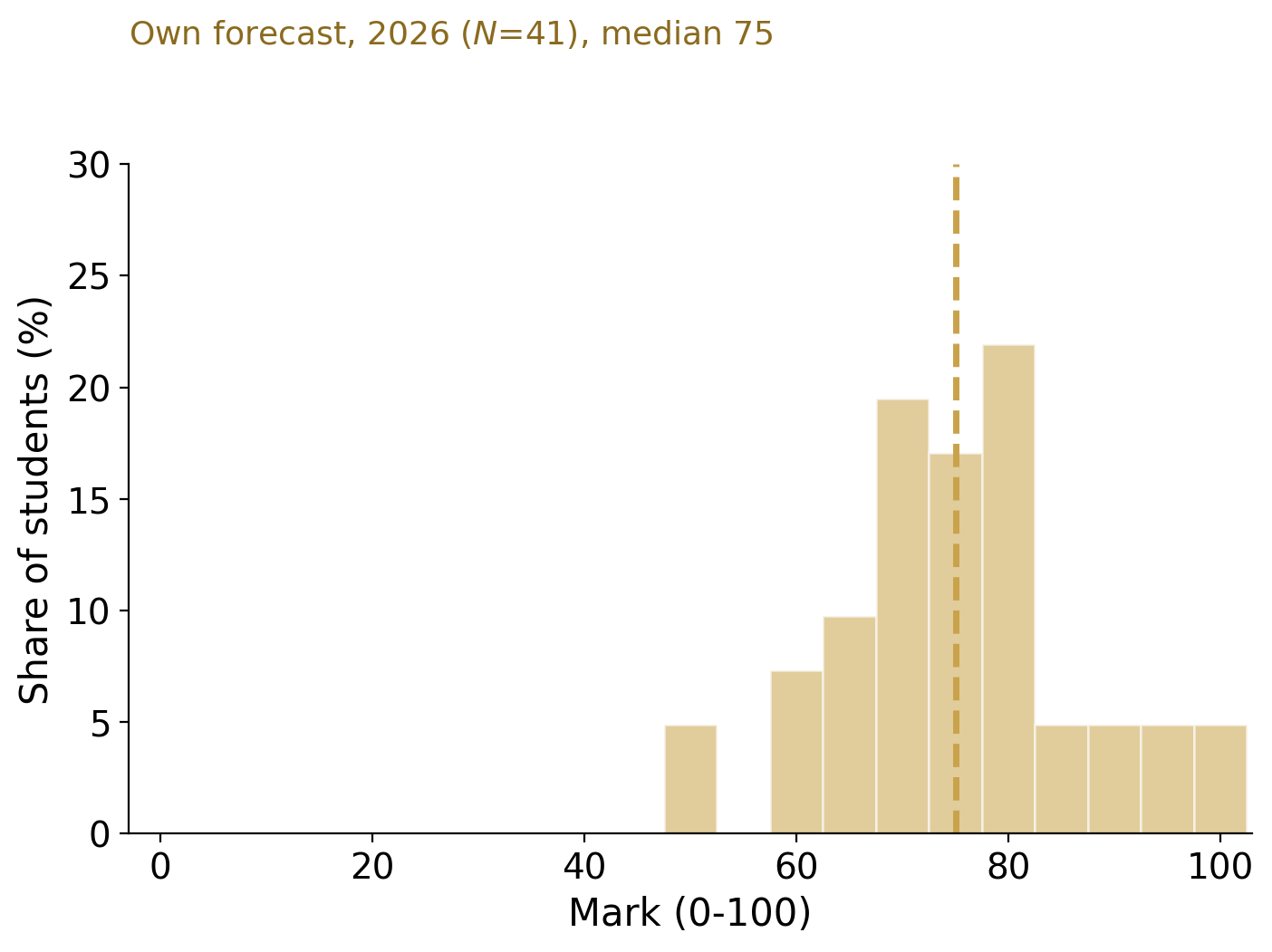
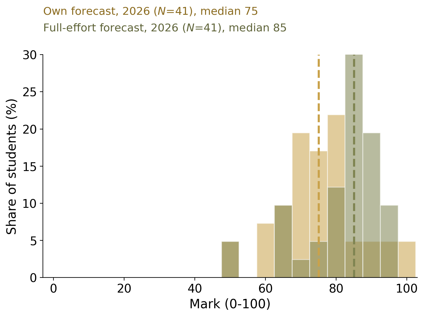
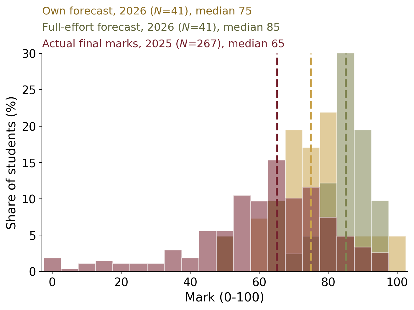
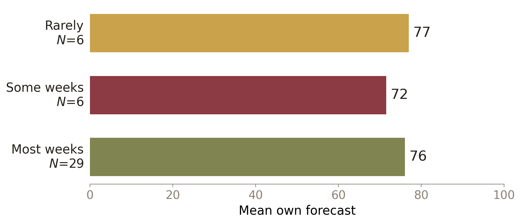
Your own semester
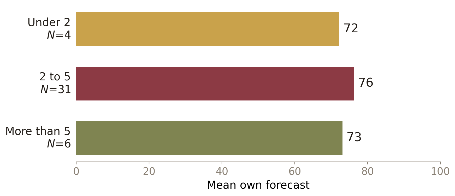
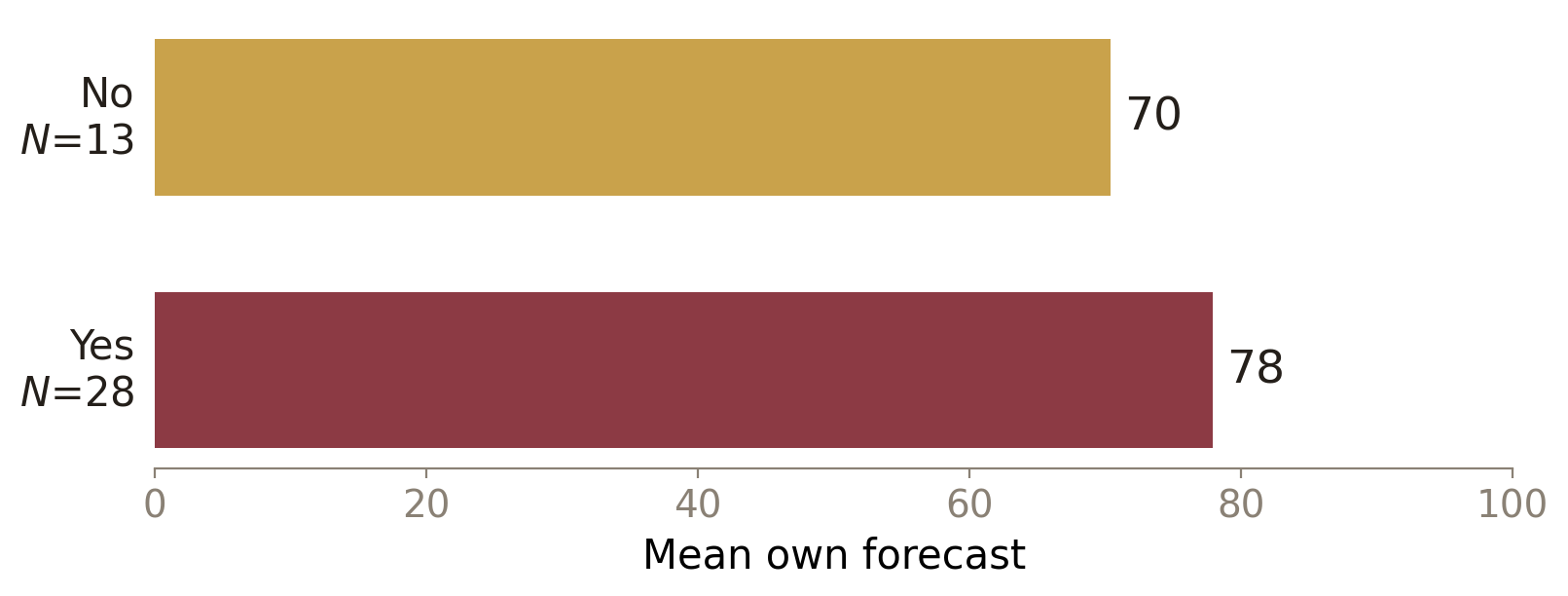
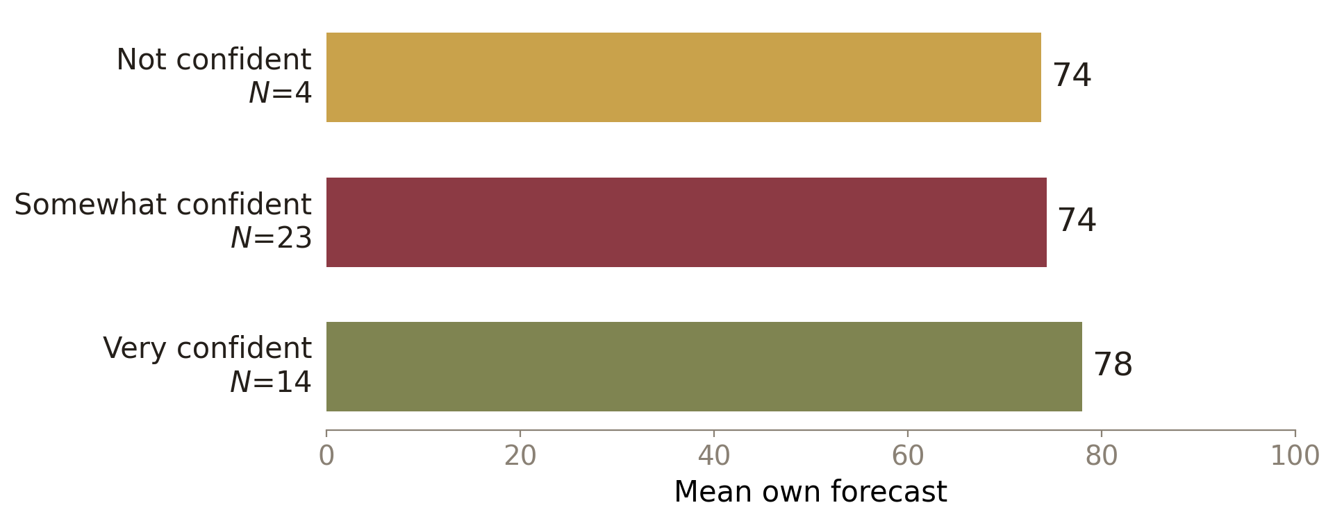
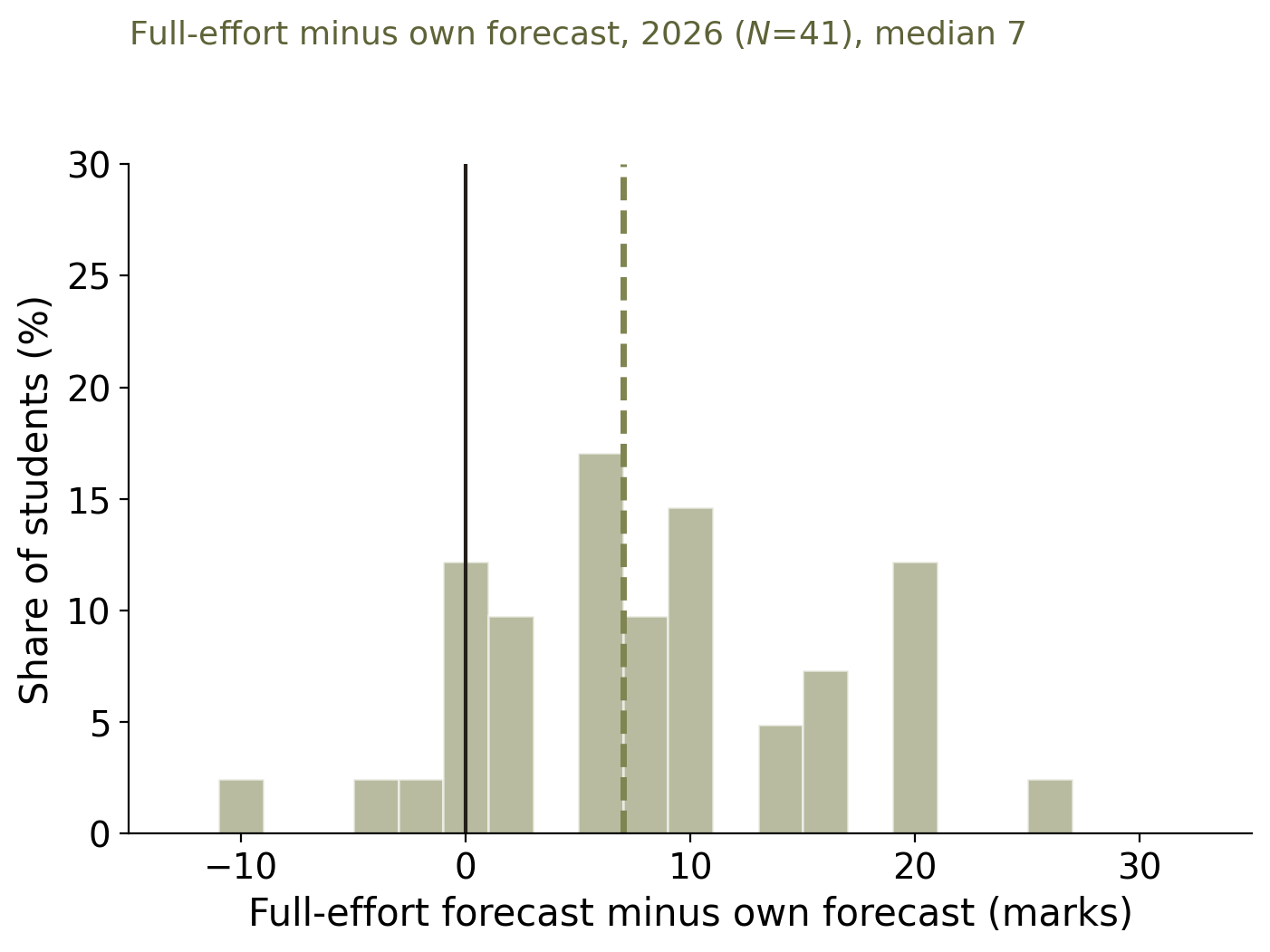
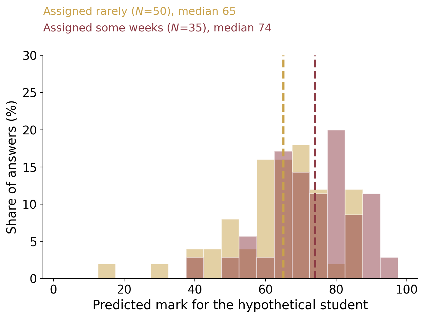
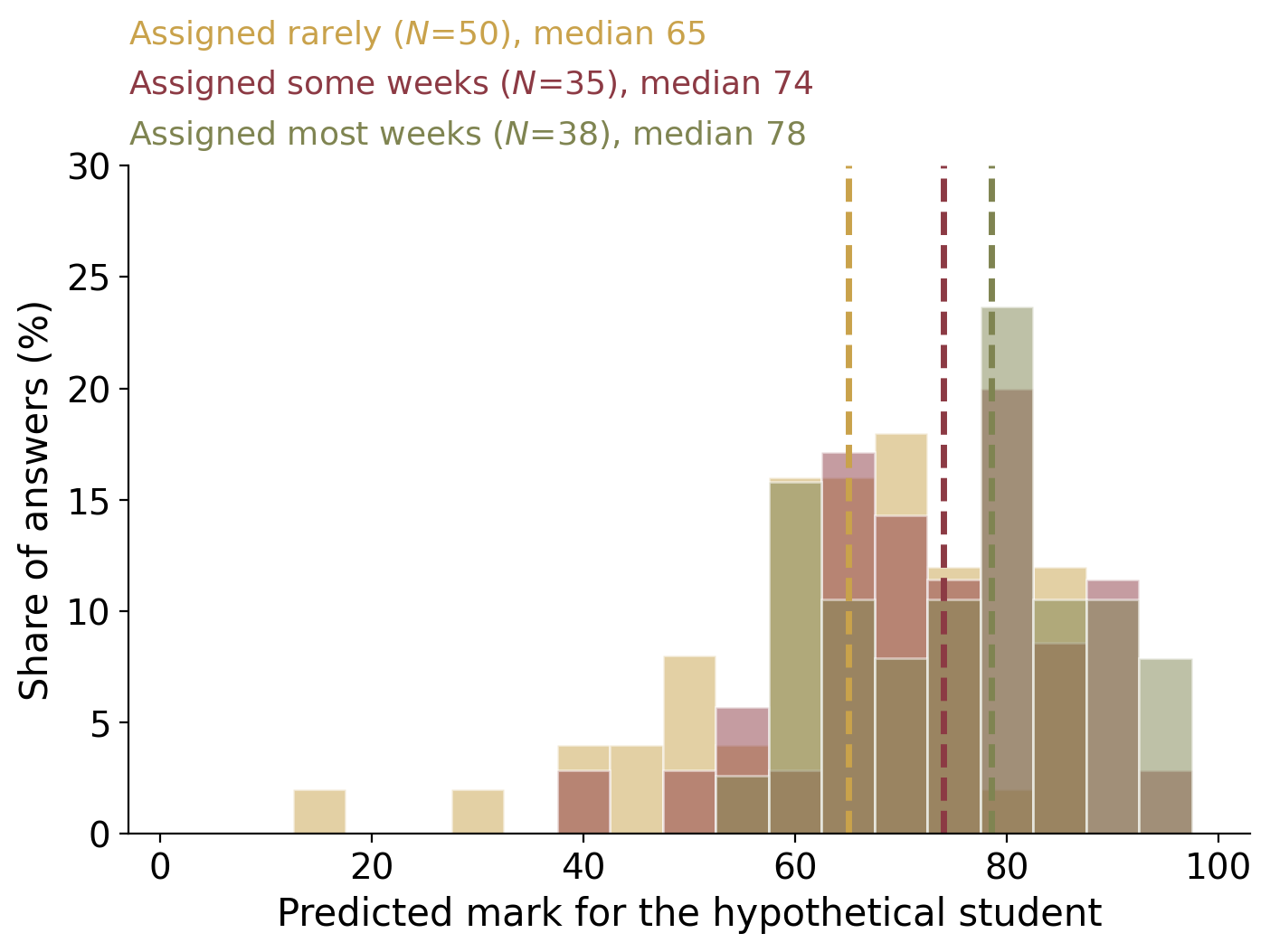
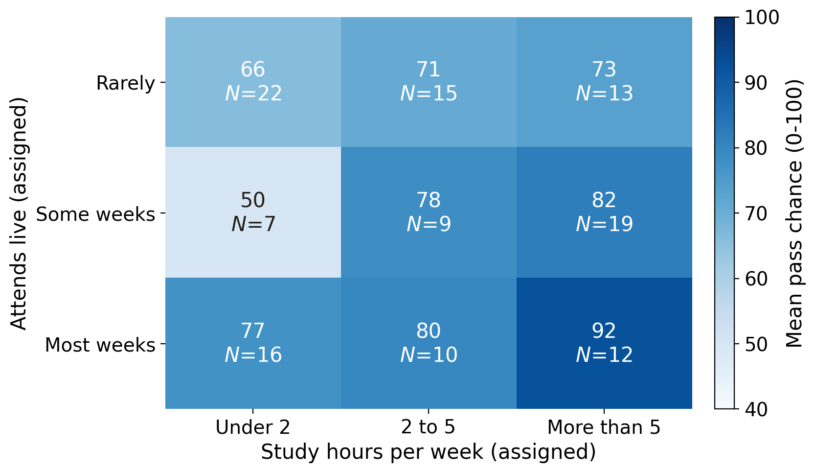
Three hypothetical students
For each:


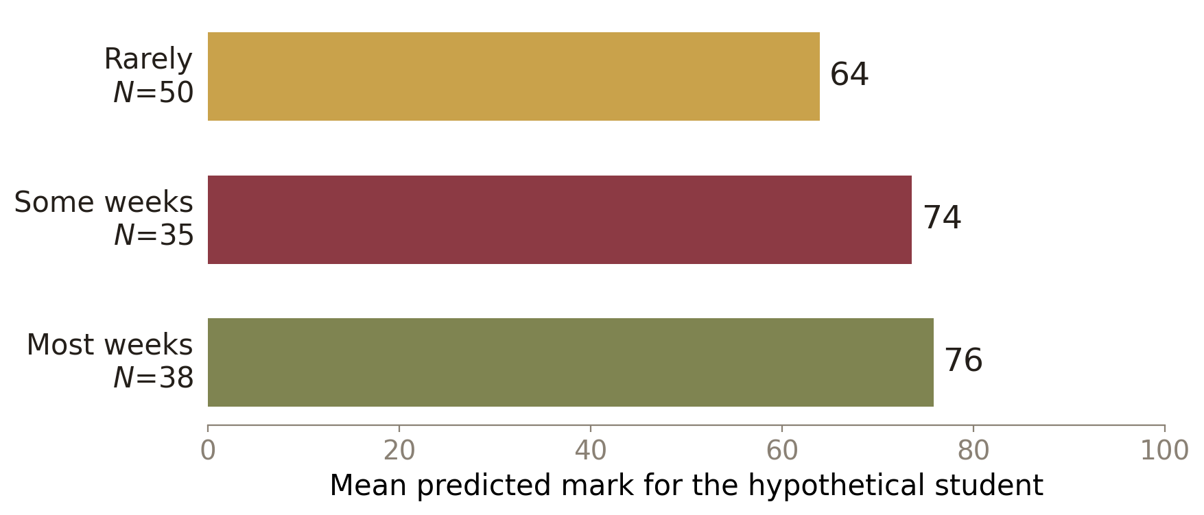
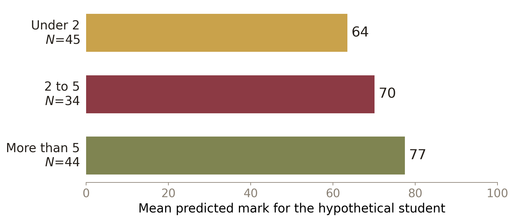
Share of hypothetical students at each study-hours level, within each attendance level
| Assigned study hours per week | ||||
|---|---|---|---|---|
| Assigned attendance | <2 | 2 - 5 | 5+ | N |
| Rarely | 44% | 30% | 26% | 50 |
| Some weeks | 20% | 26% | 54% | 35 |
| Most weeks | 42% | 26% | 32% | 38 |
| All vignettes | 37% | 28% | 36% | 123 |


For each hypothetical student, two chances:
Every mark of 75 or more is also a mark of 50 or more
\{\text{mark} \geq 75\} \subset \{\text{mark} \geq 50\}, so P(\text{mark} \geq 75) \leq P(\text{mark} \geq 50)
10 of 120 answers put the probability of D > probability of P

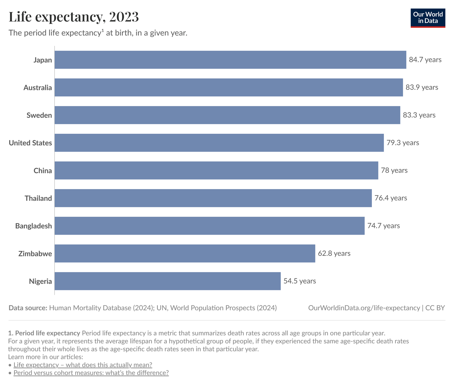
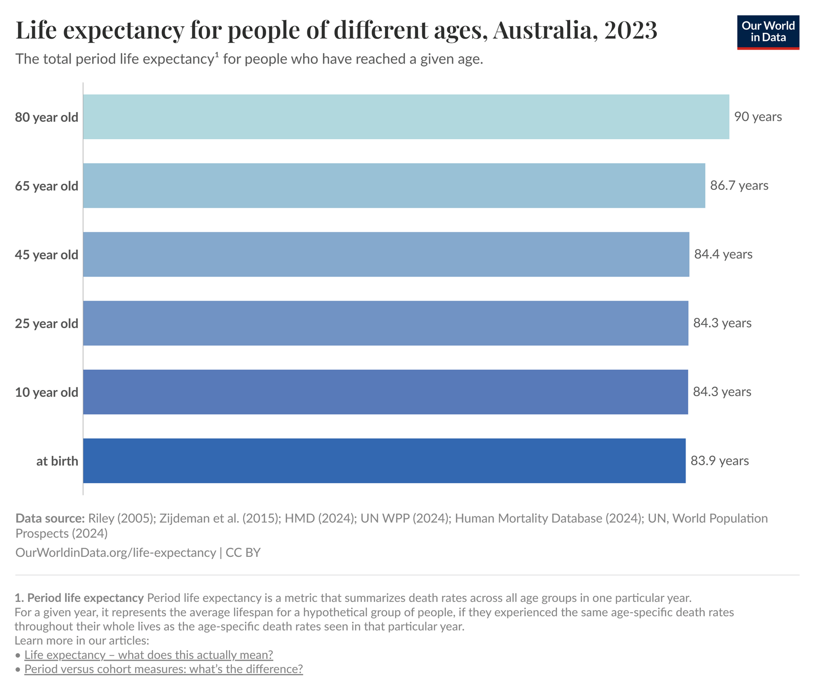
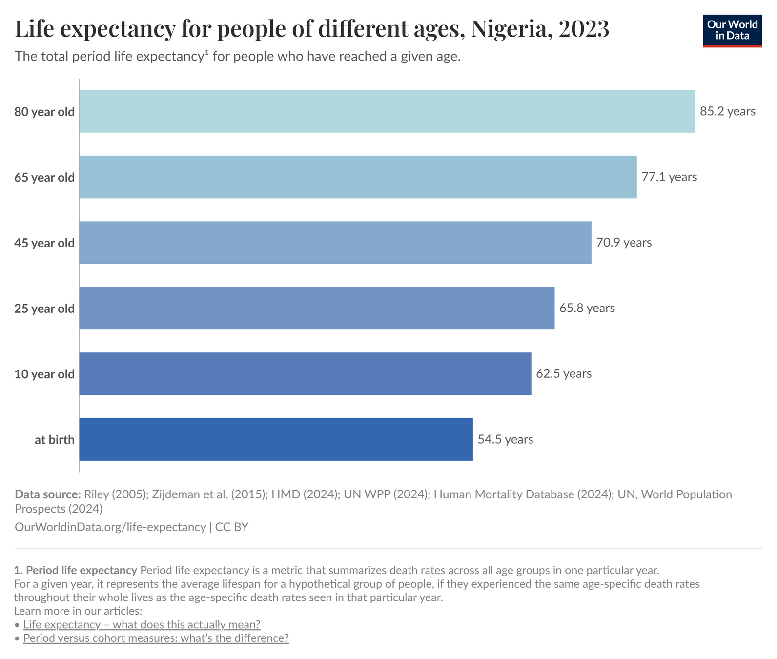
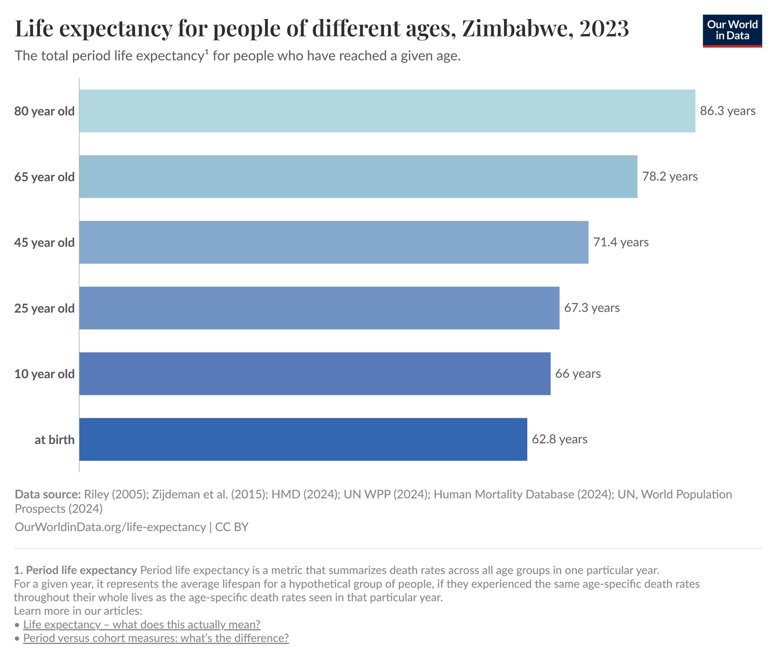
Life expectancy is based on an estimate of the average age that members of a particular population group will be when they die
Source:
Our World in Data


Source: Our World in Data
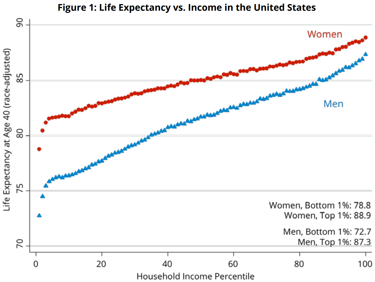
US men, aged 40, 2001 - 2014
How many more years does a man in the richest 1% expect to live than a man in the poorest 1%?

Men, age 40
Women: a gap of 10.1 years
Y: life expectancy at 40
X: income percentile
Each dot is E[Y \mid X = x]
E[Y \mid X = \text{p20}] \approx 77
E[Y \mid X = \text{p80}] \approx 84
Source: Chetty et al. (2016)

Y: life expectancy at 40
X: income percentile
Z: sex
Each line is
E[Y \mid X = x, Z = z]
Source: Chetty et al. (2016)
E[Y] hides a lot of heterogeneity that we can see with E[Y | X]!


Low-income men in the US have \approx LE as Zimbabwean men!


Does this suggest that giving more money to those at the bottom of the income distribution would \uparrow their life expectancy?
Source: Chetty et al. (2016)
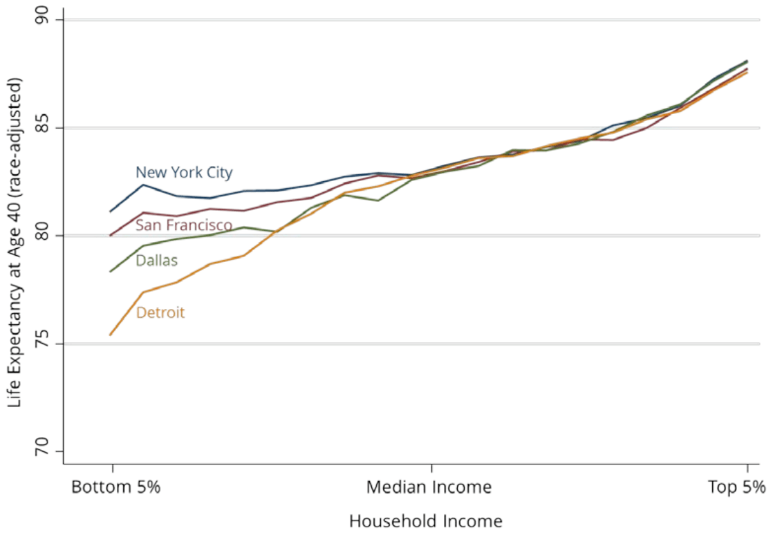
Place matters!

It's better to be poor in
New York than in Detroit
Source: Chetty et al. (2016)
Discrete: takes a finite set of values
Continuous: takes a continuum
But every column in every dataset has finitely many values
escs, the socio-economic index: 62 distinct values in 12,136 rowsmath score: 3,858 distinct valuesAsk what the variable measures in the world, not how many values the column has
| In the world | Example | Arithmetic makes sense? |
|---|---|---|
| A count | number of siblings: 0, 1, 2, ... | yes: an average of 1.4 siblings |
| A measurement | math score, socio-economic index, height | yes: any value in a range, rounded when recorded |
| A label | degree enrolled in, suburb, gender | no: there is no average suburb |
Education recorded as
df['education'].mean() returns 2.3
2.3 is a fact about the codes, not about anyone's education
Six correlations
For each one: guess the correlation

Data: PISA 2022, Australia (OECD)

Data: PISA 2022, Australia (OECD)

Data: PISA 2022, Australia (OECD)

Data: PISA 2022, Australia (OECD)

Data: Gallup World Poll & World Bank, via Our World in Data

Data: Gallup World Poll & World Bank, via Our World in Data

Data: Gallup World Poll & World Bank, via Our World in Data

Data: UN World Population Prospects, via Our World in Data

Data: UN World Population Prospects, via Our World in Data

Data: PISA 2022, Australia (OECD), 25 students drawn at random

Data: PISA 2022, Australia (OECD), 25 students drawn at random

Data: PISA 2022, Australia (OECD)


Data: PISA 2022, Australia (OECD), 300 students drawn at random

Data: PISA 2022, Australia (OECD), 300 students drawn at random


\text{cov}(X, Y) = \frac{1}{n}\sum_i (x_i - \bar{x})(y_i - \bar{y}) = 29 \;\text{index points} \times \text{score points}
r = \frac{\text{cov}(X, Y)}{s_X \, s_Y} = \frac{29}{0.78 \times 91.7} = 0.41