ECON 2041
Introductory Econometrics
Review
Plan for the semester
2 Basic mathematical tools
7 Flavors of OLS & OVB Quiz
10 Inference, continued PS due 16 Oct
12 Measurement error & IRL
Plan for today
- Where students lost marks last year
- Reading a regression table
- Interactions
- Testing a claim with a confidence interval
- Omitted variables and heteroskedasticity
- Data that you can trust
Where students lost marks last year
Interactions: writing the model, interpreting the coefficient, testing it
Testing a value other than 0 with a confidence interval
The direction of omitted variable bias, once a proxy is added
Reading a regression table
Read each slope with the other xs fixed
y = \beta_0 + \beta_1 x_1 + \beta_2 x_2 + u
\beta_1: average difference in y per 1 unit of x_1, holding x_2 fixed
Dummy x_2: average difference in y between groups 1 and 0, holding x_1 fixed
Airbnb prices: guests, rating, entire home
ols("price ~ guests + rating + entire_home", data=airbnb).fit(cov_type="HC3")
                  coef    std err          z      P>|z|      [0.025      0.975]
-------------------------------------------------------------------------------
Intercept    -269.6861     27.520     -9.800      0.000    -323.623    -215.749
guests         63.8244      1.357     47.023      0.000      61.164      66.485
rating         63.8766      6.005     10.638      0.000      52.108      75.646
entire_home   100.2121      4.231     23.686      0.000      91.920     108.504
entire_home = 1 for an entire home or apartment, 0 for a room
Data: Inside Airbnb, Sydney, snapshot of 16 June 2026; 12,419 listings
Open the portal on your phone
On the next slide: 4 sentences about the coefficient on entire_home in our Airbnb regression
Pick the one that's right
https://emiliatjernstrom.com/econ2041/portal.html
Reading the entire-home coefficient
\text{price} = \beta_0 + \beta_1\,\text{guests} + \beta_2\,\text{rating} + \beta_3\,\text{entire} + u
entire = 1 for an entire home, 0 for a room; \hat{\beta}_3 = 100.21
In all 4, guests and rating are held fixed
A. An entire home costs $100.21 a night, on average
B. An entire home costs $100.21 more a night than a room, on average \leftarrow
C. Turning a room into an entire home raises its price by $100.21 a night
D. An entire home costs 100.21% more a night than a room, on average
On the portal, open W13 dummy coefficient: https://emiliatjernstrom.com/econ2041/portal.html
Log price: coefficient \times 100 \approx % difference
ols("np.log(price) ~ guests + rating + entire_home",
    data=airbnb).fit(cov_type="HC3")
                  coef    std err          z      P>|z|      [0.025      0.975]
-------------------------------------------------------------------------------
Intercept       3.9228      0.059     66.401      0.000       3.807       4.039
guests          0.1299      0.002     59.573      0.000       0.126       0.134
rating          0.1585      0.013     12.125      0.000       0.133       0.184
entire_home     0.6012      0.015     39.382      0.000       0.571       0.631
1 more guest: about 100 \times 0.13 = 13\% higher price, holding rating and entire home fixed
Data: Inside Airbnb, Sydney, snapshot of 16 June 2026; 12,419 listings
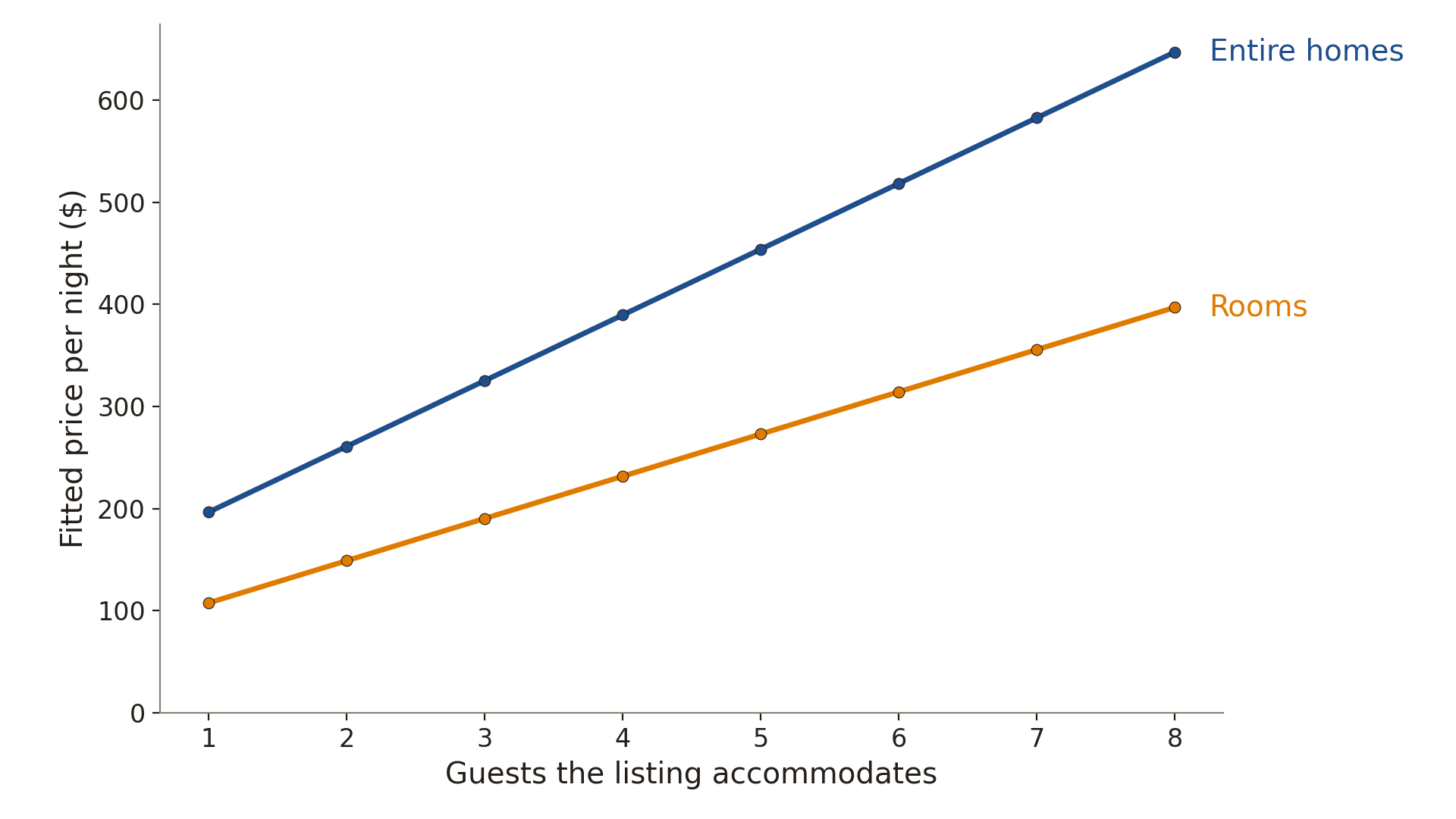
With an interaction, slopes differ by group
\text{price} = \beta_0 + \beta_1\,\text{guests} + \beta_2\,\text{entire} + \beta_3\,(\text{guests} \times \text{entire}) + u
Rooms, entire = 0: slope on guests is \beta_1
Entire homes, entire = 1: slope on guests is \beta_1 + \beta_3
\beta_3: how much larger the slope is for entire homes than for rooms
Interactions in Python: a colon
ols("price ~ guests + entire_home + guests:entire_home",
    data=airbnb).fit(cov_type="HC3")
                         coef    std err          z      P>|z|      [0.025      0.975]
--------------------------------------------------------------------------------------
Intercept             66.0203     12.544      5.263      0.000      41.435      90.605
guests                41.3797      6.030      6.862      0.000      29.561      53.199
entire_home           65.9176     13.653      4.828      0.000      39.157      92.678
guests:entire_home    23.0458      6.190      3.723      0.000      10.913      35.179
Data: Inside Airbnb, Sydney, snapshot of 16 June 2026; 12,419 listings
Reading the interaction coefficient
\text{price} = \beta_0 + \beta_1\,\text{guests} + \beta_2\,\text{entire} + \beta_3\,(\text{guests} \times \text{entire}) + u
\hat{\beta}_3 = 23.05
A. For entire homes, the slope on guests is $23.05 per guest
B. Entire homes have a slope on guests $23.05 steeper than rooms \leftarrow
C. Entire homes cost $23.05 more a night than rooms, holding guests fixed
D. Each extra guest is associated with a price $23.05 higher for every listing
On the portal, open W13 interaction coefficient: https://emiliatjernstrom.com/econ2041/portal.html
Two slopes from one regression
Data: Inside Airbnb, Sydney, snapshot of 16 June 2026; 12,419 listings; fitted values for 1 to 8 guests
Is the slope different for entire homes?
H_0: \beta_3 = 0 \qquad H_A: \beta_3 \neq 0
95% confidence interval for \beta_3: 10.91 to 35.18
0 is outside the confidence interval, so we reject H_0 at the 5% level
Three tools, three questions
| 1 coefficient equal to a value? |
t-test |
p < \alpha |
| Plausible values of 1 coefficient? |
Confidence interval |
Value outside it |
| Several coefficients all 0? |
F-test |
p < \alpha |
A host claims a $65 gap per extra guest
From our first table: coefficient on guests 63.82, 95% confidence interval 61.16 to 66.49
A. Reject: 65 isn't equal to the estimate, 63.82
B. Don't reject: 65 is inside the 95% confidence interval \leftarrow
C. Reject: the p-value for guests, 0.000, is below 0.05
D. Can't tell: the table's p-value is for 0 only
On the portal, open W13 testing a host's claim: https://emiliatjernstrom.com/econ2041/portal.html
Test any value with a confidence interval
$65: inside 61.16 to 66.49, so we don't reject
$70: outside, so we reject at the 5% level
Not rejecting $65 doesn't show that $65 is true
Two conditions for omitted variable bias
The omitted variable affects y, holding x fixed
The omitted variable is correlated with x
| Affects y + |
Bias + |
Bias − |
| Affects y − |
Bias − |
Bias + |
Pokies: which way is the omitted variable bias?
Losses per adult on pokies per 1,000 adults: slope 78.3
Unemployment affects losses: +
Unemployment is correlated with pokie density: +
Positive bias: the slope is 72.8 with unemployment in the regression
Data: VGCCC 2024, 79 Victorian LGAs
Heteroskedasticity: invalid standard errors
The error variance differs across observations
Usual standard errors are invalid: use robust ones, cov_type="HC3"
Data: Inside Airbnb, Sydney, snapshot of 16 June 2026; 12,419 listings
Three ways data go wrong
Structure: 1 row per observation, 1 column per variable
Quality: the values themselves are wrong, such as -999 for missing, duplicates, mixed units
Measurement: the recorded values have error
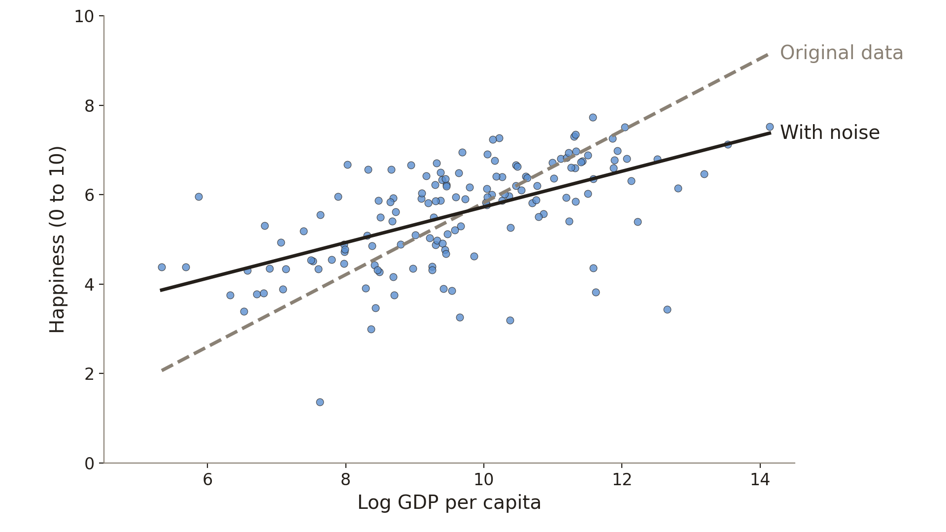
With which noise is the slope flatter?
On the portal, open W13 noise in X or Y
I'll add random noise to 1 variable
A. Only noise in happiness scores (y)
B. Only noise in log GDP (x) \leftarrow
C. Noise in either of the variables
D. Neither of the two kinds of noise
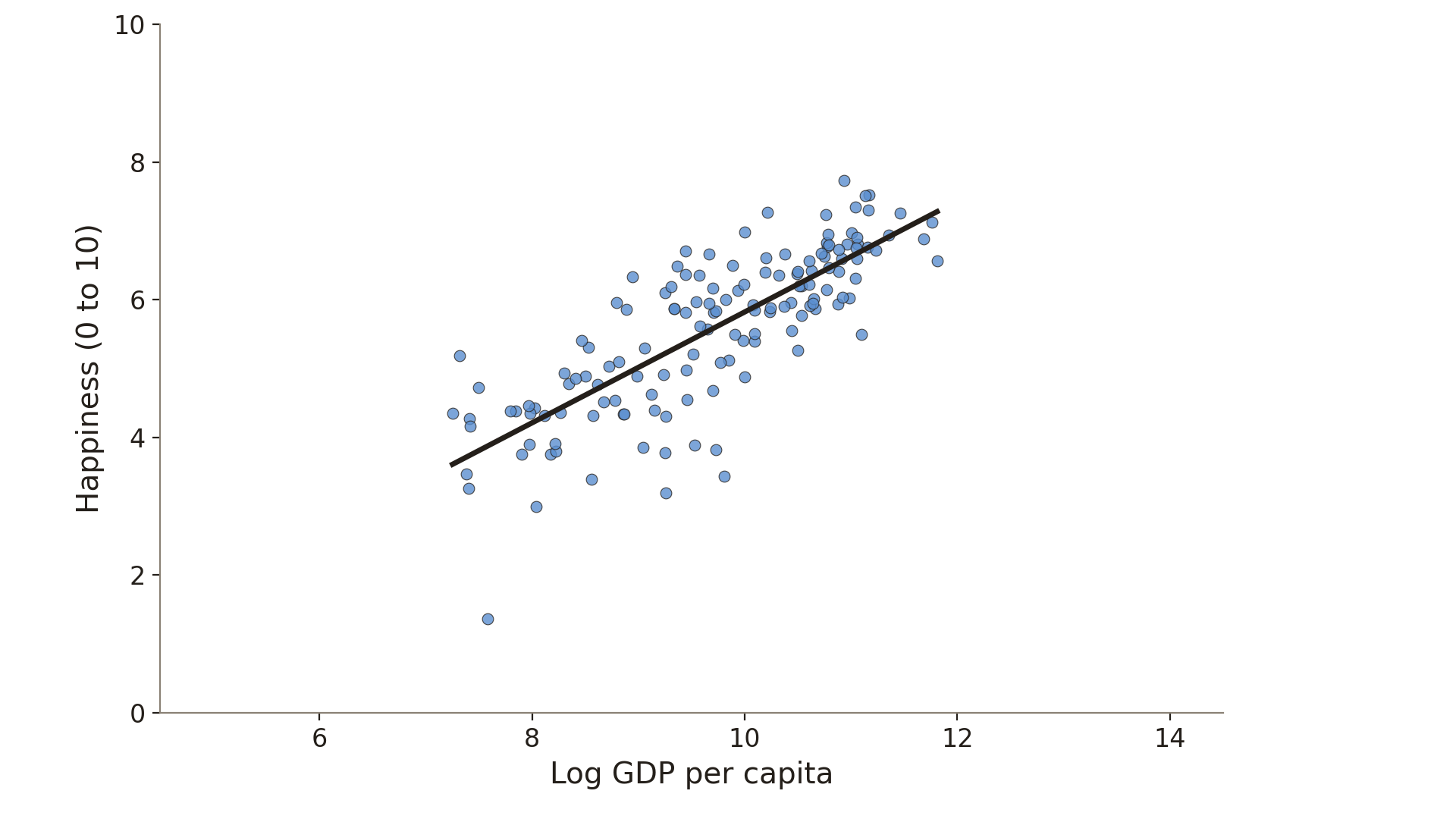
Data: Gallup World Poll & World Bank, via Our World in Data; 144 countries, 2024
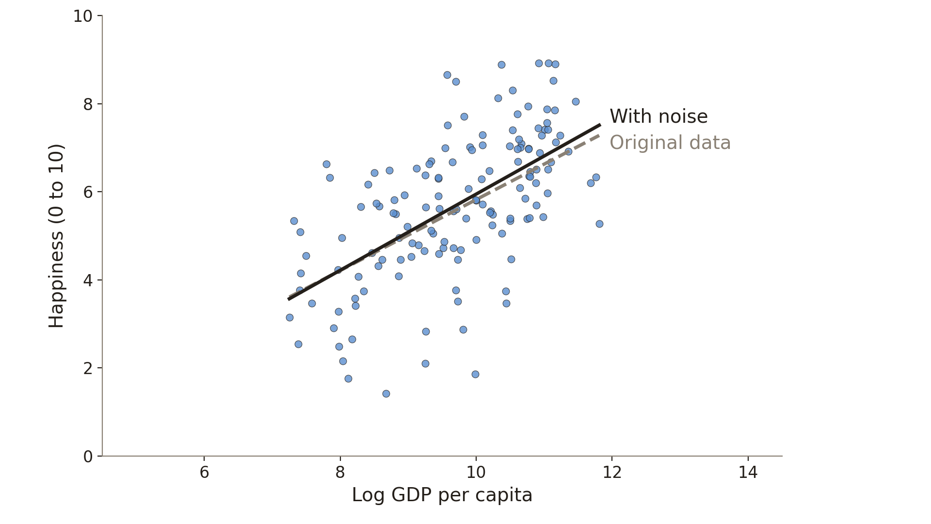
Noise in y: similar slope, larger standard error
Data: Gallup World Poll & World Bank, via Our World in Data; 144 countries, 2024; noise added to happiness
Noise in x: a flatter slope
Data: Gallup World Poll & World Bank, via Our World in Data; 144 countries, 2024; noise added to log GDP