ECON 2041
Introductory Econometrics
More than one X
Plan for the semester
1 What is econometrics?
2 Basic mathematical tools
3 Stats fundamentals
4 Stats fundamentals II
5 Simple regression
6 OLS properties & fit
7 Flavors of OLS & OVB Quiz
8 Causality
9 Regression inference
10 Inference, continued PS due 16 Oct
11 Diagnostics
12 Measurement error & IRL
13 Revision
Plan for today
- Pokies and losses across 79 LGAs
- Unemployment, holding pokie density fixed
- Letting the slopes differ: interactions
- The problem set, in brief
- More than two categories
Pokie density correlated w/ gambling losses
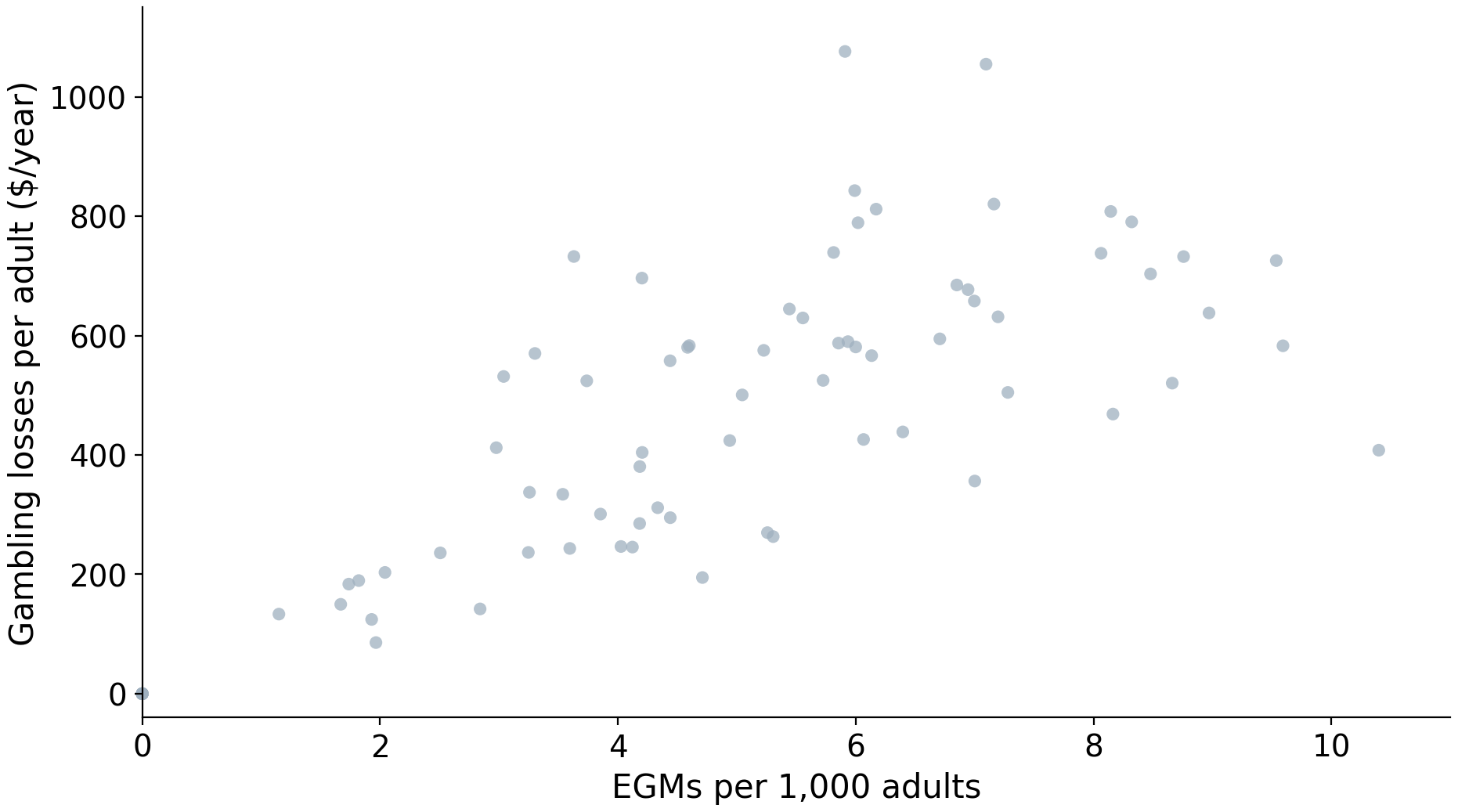
Data: VGCCC 2024, 79 Victorian LGAs
What the correlation misses
How many dollars per pokie?
Same method as before
New data
You can follow along in a notebook
https://emiliatjernstrom.com/econ2041/lectures/w08
As usual, it will open directly in Colab
Click Copy to Drive first, so you can save your edits
OLS output: slope & intercept
from statsmodels.formula.api import ols

model = ols("exp_per_adult ~ egm_per_1000", data=pokies).fit()
coef std err t P>|t| [0.025 0.975]
--------------------------------------------------------------------------------
Intercept 71.1722 38.992 1.825 0.072 -6.471 148.816
egm_per_1000 78.2968 7.205 10.866 0.000 63.949 92.645OLS confirms: more pokies, more losses
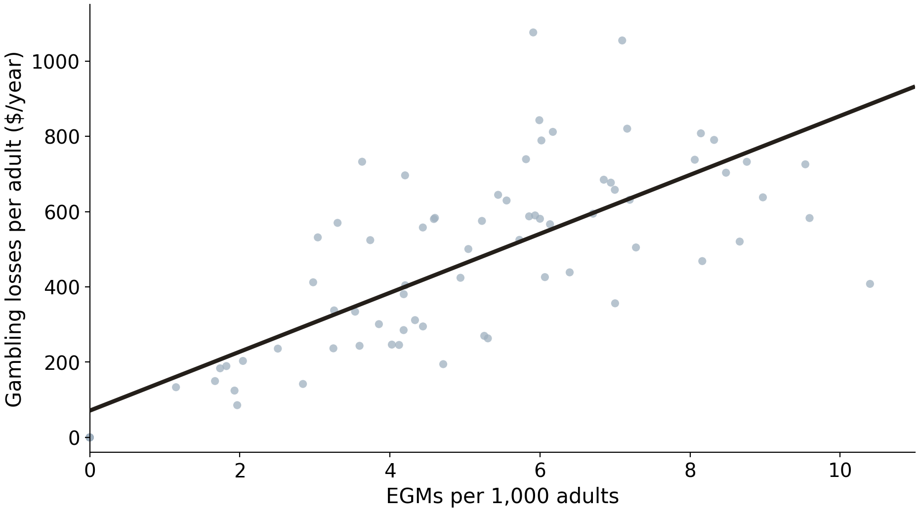
\widehat{\text{losses}} = 71 + 78 \times \text{EGMs per 1,000}
Data: VGCCC 2024, 79 Victorian LGAs
Is unemployment pokie density in disguise?
Our simple regression conditioned on one variable
Take 2 LGAs with the same pokie density, one high-unemployment and one low: does the high one still lose more?
E[\,\text{losses} \mid \text{EGMs}, \text{unemployment} = \text{high}\,]
E[\,\text{losses} \mid \text{EGMs}, \text{unemployment} = \text{low}\,]
A dummy variable encodes a category as 0 or 1
median_val = pokies["ue_rate"].median()
pokies["high_ue"] = (pokies["ue_rate"] > median_val).astype(int)
high_ue stores the answer to our comparison
.astype(int) turns True/False into 1 and 0: 1 means above-median unemployment (39 LGAs), 0 means below-median (40 LGAs)
A 0/1 variable is called a dummy variable
Unemployment is not pokie density in disguise
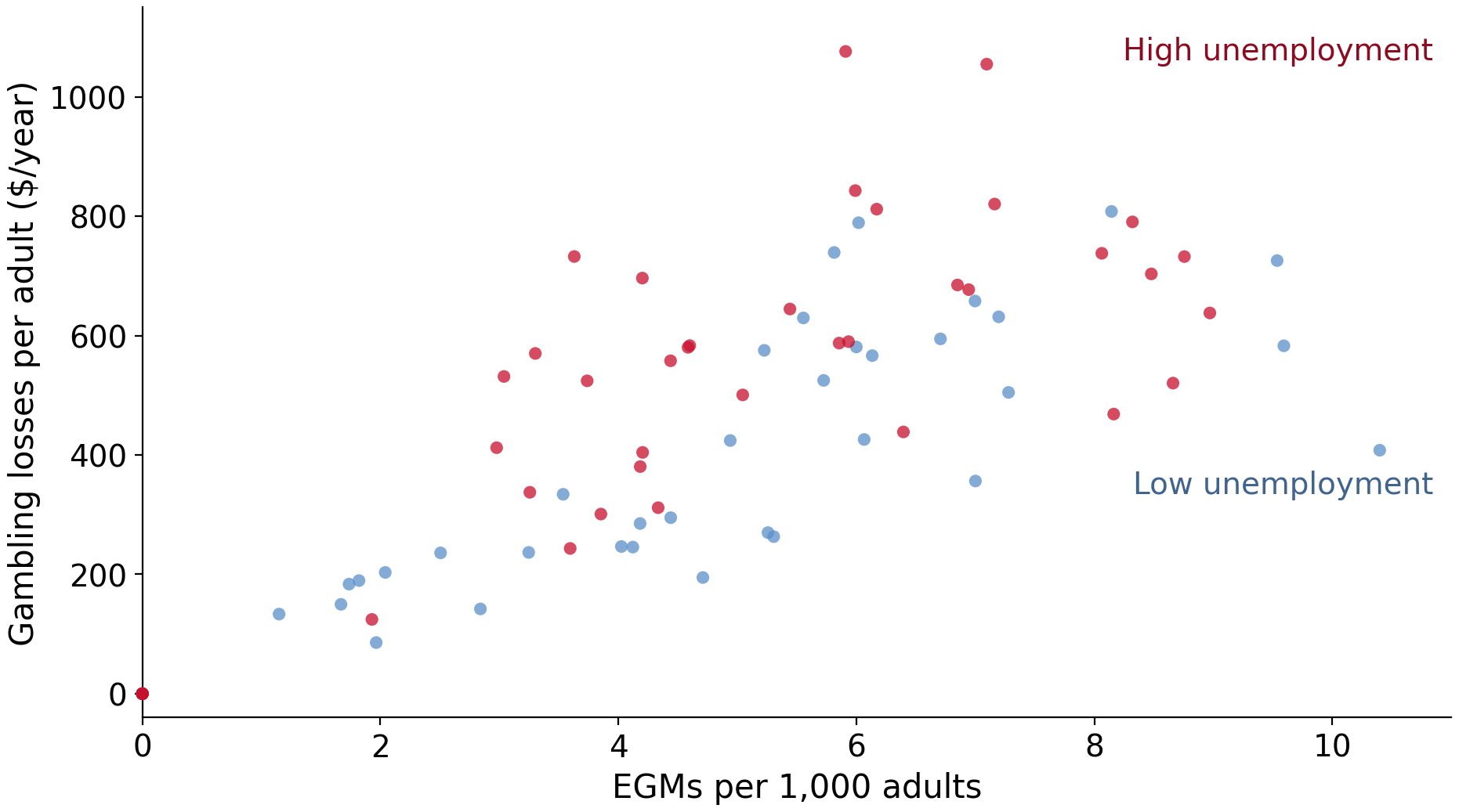
Data: VGCCC 2024, 79 Victorian LGAs
Unemployment is not pokie density in disguise
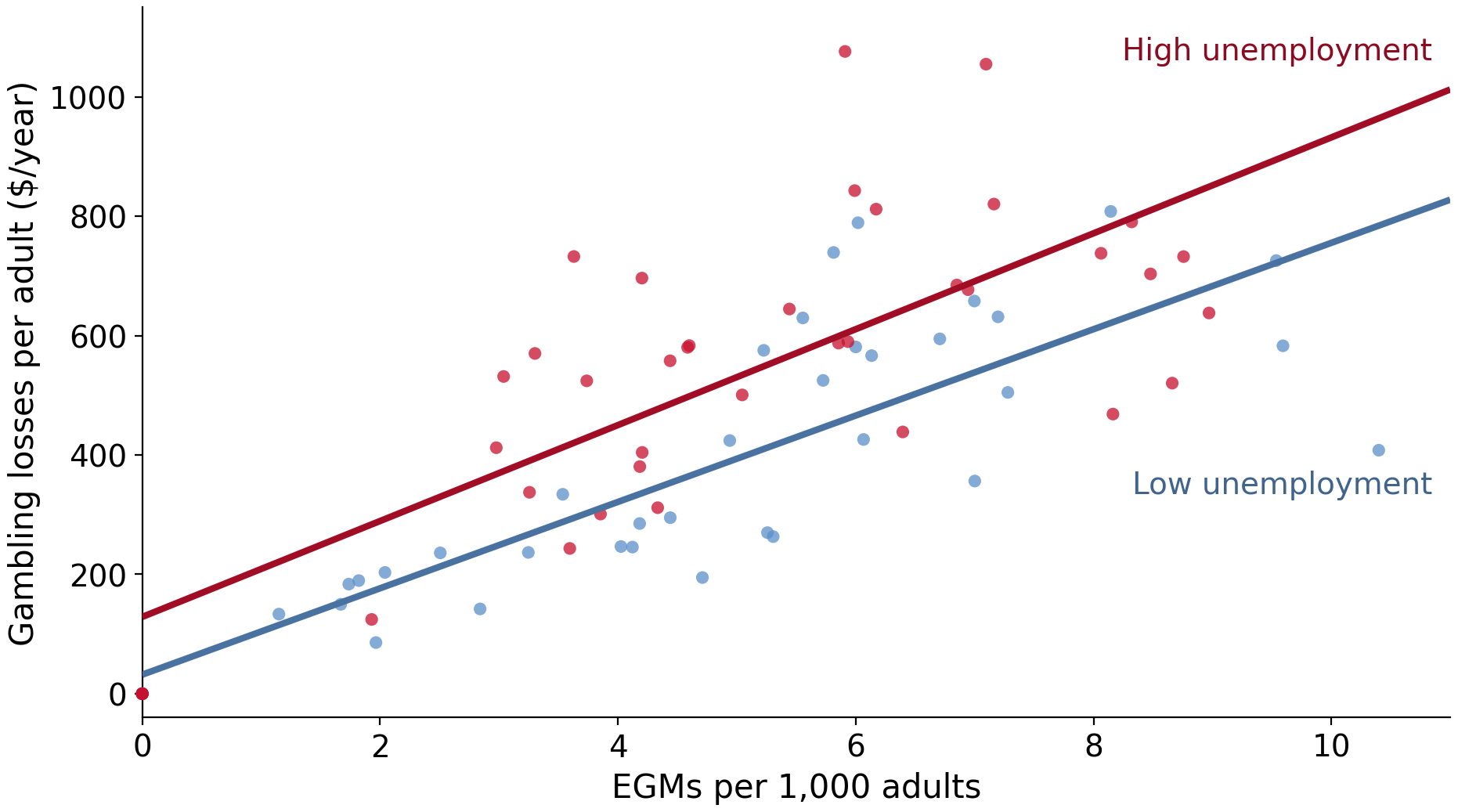
Data: VGCCC 2024, 79 Victorian LGAs
Multiple regression!
Instead of splitting the sample,
put both variables in one regression
and use all 79 LGAs
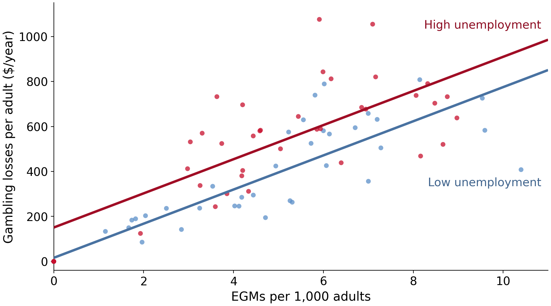
The dummy shifts the intercept
\text{losses}_i = \beta_0 + \beta_1 \, \text{EGMs}_i + \beta_2 \, \text{high\_ue}_i + u_i
For low-unemployment LGAs (\text{high\_ue} = 0): intercept \beta_0
For high-unemployment LGAs (\text{high\_ue} = 1): intercept \beta_0 + \beta_2
Same slope \beta_1 in both groups: two parallel lines
Add the high-unemployment dummy
                   coef    std err          t      P>|t|      [0.025      0.975]
--------------------------------------------------------------------------------
Intercept       16.1362     38.739      0.417      0.678     -61.018      93.291
egm_per_1000    75.8681      6.674     11.367      0.000      62.575      89.161
high_ue        134.7112     35.300      3.816      0.000      64.406     205.016
The gap is the same at every pokie density
Data: VGCCC 2024, 79 Victorian LGAs
Separate slopes or one shared slope?
Two regressions, two slopes
One regression, one shared slope
Data: VGCCC 2024, 79 Victorian LGAs
The second X can be continuous
pokies["ue_pct"] = 100 * pokies["ue_rate"]
ols("exp_per_adult ~ egm_per_1000 + ue_pct", data=pokies).fit()
coef std err t P>|t| [0.025 0.975]
--------------------------------------------------------------------------------
Intercept -115.9316 49.520 -2.341 0.022 -214.559 -17.304
egm_per_1000 72.8291 6.329 11.507 0.000 60.224 85.434
ue_pct 61.1848 11.845 5.165 0.000 37.593 84.776Why use one regression instead of splitting?
Uses all the data for every coefficient \rightarrow more precise estimates
Holds the other X fixed: but only the variables we put in the formula
Scales: if we have 3, 4, or 10 X-variables, splitting would not work!
Letting the slopes differ
One regression
Two intercepts
Two slopes
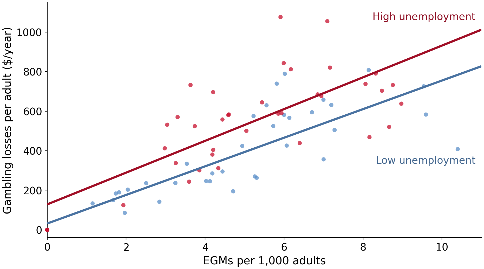
Two groups, two slopes, one regression
\text{losses}_i = \beta_0 + \beta_1 \, \text{EGMs}_i + \beta_2 \, \text{high\_ue}_i + \beta_3 \, (\text{EGMs}_i \times \text{high\_ue}_i) + u_i
Low unemployment (\text{high\_ue} = 0): intercept \beta_0, slope \beta_1
High unemployment (\text{high\_ue} = 1): intercept \beta_0 + \beta_2, slope \beta_1 + \beta_3
\beta_3 is the difference in slopes between the two groups
In a formula, a colon means interaction
                           coef    std err          t      P>|t|      [0.025      0.975]
----------------------------------------------------------------------------------------
Intercept               31.9430     47.186      0.677      0.501     -62.056     125.942
egm_per_1000            72.3339      8.976      8.058      0.000      54.453      90.215
high_ue                 96.7287     73.302      1.320      0.191     -49.296     242.753
egm_per_1000:high_ue     7.9900     13.496      0.592      0.556     -18.896      34.876
Same fitted values as the split sample
Data: VGCCC 2024, 79 Victorian LGAs
An asterisk is shorthand for all three terms
                           coef    std err          t      P>|t|      [0.025      0.975]
----------------------------------------------------------------------------------------
Intercept               31.9430     47.186      0.677      0.501     -62.056     125.942
egm_per_1000            72.3339      8.976      8.058      0.000      54.453      90.215
high_ue                 96.7287     73.302      1.320      0.191     -49.296     242.753
egm_per_1000:high_ue     7.9900     13.496      0.592      0.556     -18.896      34.876
a * b means a + b + a:b, so an interaction never enters without its parts
The problem set, in brief
30% of your grade
Opens Friday 2 October at 9:00, due Friday 16 October at 23:55
- complete it in an iLearn "quiz"
- a short memo
- your notebook
Covers material through week 9
More than two categories
Low, medium, high
One formula
Which numbers?
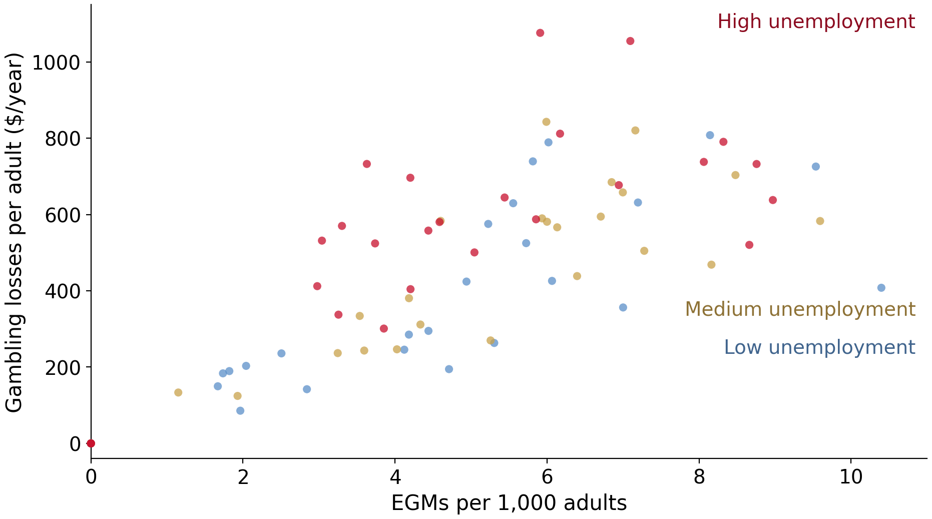
Three equal-sized unemployment groups
pokies["ue_cat"] =  pd.qcut(pokies["ue_pct"], 3,
                    labels=["low", "medium", "high"])
pokies["ue_cat"].value_counts()
ue_cat
low 27
medium 26
high 26
Name: count, dtype: int64pd.qcut cuts at the tertiles (2.9% and 4.0%) so the groups are of equal size
Low & medium unemployment look alike
Data: VGCCC 2024, 79 Victorian LGAs
Categories have no units, so no single slope
# low = 1, medium = 2, high = 3
pokies["ue_code"] = pokies["ue_cat"].cat.codes + 1
ols("exp_per_adult ~ egm_per_1000 + ue_code", data=pokies).fit()
coef std err t P>|t| [0.025 0.975]
--------------------------------------------------------------------------------
Intercept -85.6603 53.995 -1.586 0.117 -193.201 21.881
egm_per_1000 76.4537 6.642 11.511 0.000 63.225 89.682
ue_code 83.2945 21.444 3.884 0.000 40.585 126.004One coefficient forces the medium-to-high gap to equal the low-to-medium gap
One dummy per category, minus one
                          coef    std err          t      P>|t|      [0.025      0.975]
---------------------------------------------------------------------------------------
Intercept              13.2748     41.581      0.319      0.750     -69.558      96.108
C(ue_cat)[T.medium]    28.5316     42.573      0.670      0.505     -56.279     113.342
C(ue_cat)[T.high]     167.0544     42.553      3.926      0.000      82.284     251.825
egm_per_1000           76.9259      6.597     11.660      0.000      63.783      90.069
Low = reference category
i.e., each coefficient is a gap relative to low, at the same pokie density
Three intercepts, one shared slope
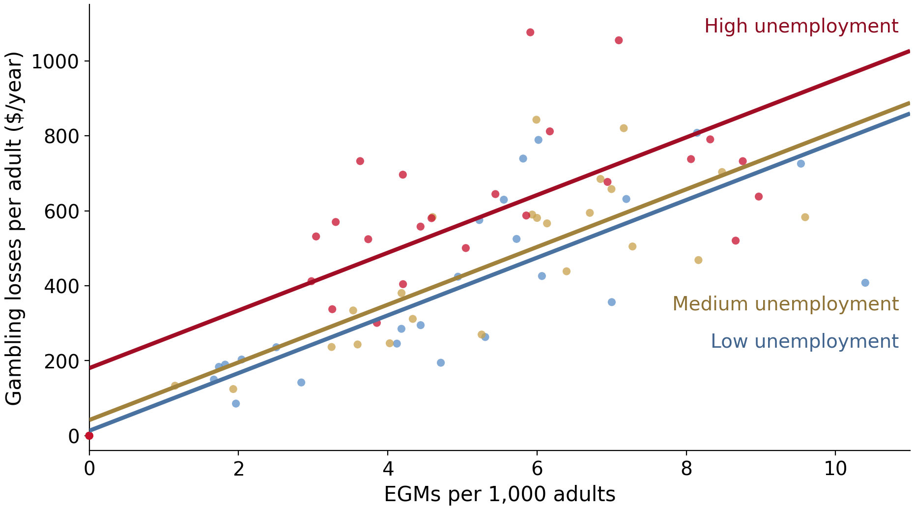
\widehat{\text{losses}} = 13 + 77 \times \text{EGMs} + 29 \times \text{medium} + 167 \times \text{high}
Data: VGCCC 2024, 79 Victorian LGAs
The pokie slope is similar in every model
summary_col([model, multi, multi_ue, levels, inter], stars=True, float_format="%.2f",
            model_names=["Simple", "Dummy", "Percent", "3 levels", "Interaction"])
Simple Dummy Percent 3 levels Interaction
----------------------------------------------------------------------------
Intercept 71.17* 16.14 -115.93** 13.27 31.94
(38.99) (38.74) (49.52) (41.58) (47.19)
egm_per_1000 78.30*** 75.87*** 72.83*** 76.93*** 72.33***
(7.21) (6.67) (6.33) (6.60) (8.98)
high_ue 134.71*** 96.73
(35.30) (73.30)
ue_pct 61.18***
(11.85)
C(ue_cat)[T.medium] 28.53
(42.57)
C(ue_cat)[T.high] 167.05***
(42.55)
egm_per_1000:high_ue 7.99
(13.50)
R-squared 0.61 0.67 0.71 0.68 0.67
R-squared Adj. 0.60 0.66 0.70 0.67 0.66Holding fixed only works for what we measured
The slope on pokie density: 78 alone, 76 with the dummy, 73 with the percentage
Each extra variable holds fixed one more thing, and only that one thing
Remoteness, venue rules: unmeasured, so still in the slope