ECON 2041
Introductory Econometrics
Can we trust these data?
Plan for the semester
1 What is econometrics?
2 Basic mathematical tools
3 Stats fundamentals
4 Stats fundamentals II
5 Simple regression
6 OLS properties & fit
7 Flavors of OLS & OVB Quiz
8 Causality
9 Regression inference
10 Inference, continued PS due 16 Oct
11 Diagnostics
12 Measurement error & IRL
13 Revision
Plan for today
- A spreadsheet from Fiji
- Three ways data go wrong
- Spot the problems
- Do messy data change our tests?
A spreadsheet from Fiji
Where would cyclone insurance have paid out?
Fiji, 1979 to 2022
Insurance that pays out when a cyclone hits
We wanted our sample to include the places cyclones hit hardest
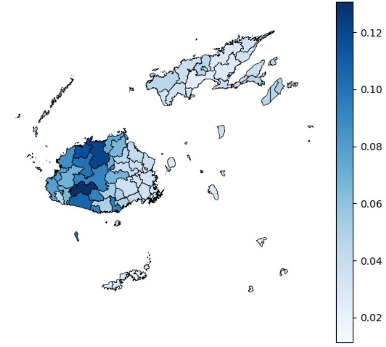
So we needed a map: 1 row per tikina, with its average payout share
The data arrived with labels stacked in rows
| Country | Fiji | Fiji | Fiji | Fiji |
|---|---|---|---|---|
| Division | Western | Western | Western | Western |
| Province | Ba | Ba | Ba | Nadroga-Navosa |
| Tikina | Nadi | Vuda | Nawaka | Cuvu |
| Beneficiaries | 18,240 | 9,615 | 3,870 | 6,105 |
| 1979 | 0.00 | 0.00 | 0.00 | 0.00 |
| 1980 | 0.05 | 0.00 | 0.08 | 0.00 |
| 1981 | 0.00 | 0.00 | 0.00 | 0.00 |
| 1982 | 0.00 | 0.00 | 0.00 | 0.12 |
| 1983 | 0.42 | 0.38 | 0.35 | 0.21 |
| 1984 | 0.00 | 0.00 | 0.00 | 0.00 |
| ⋮ | ⋮ | ⋮ | ⋮ | ⋮ |
- What is 1 observation in this sheet?
- If pandas read this sheet, what would the column names be?
- How would you average the payout share in Ba province?
Layout of the government spreadsheet; the data are confidential
Matching names to the map was painful
Move the label rows into columns
Match tikina names to the map
Average across years
Make the map
Three ways data go wrong
Rows are observations, columns are variables
1 row per observation, 1 column per variable
Python's ols expects this shape
The Fiji sheet had its labels in rows and its tikinas in columns
Quality: the values themselves are wrong
Missing values coded as -999
Duplicated rows
Mixed units, such as percent and shares
Typos
Measurement: the recorded values have error
Crop yield = harvest / field size
Farmers round field sizes: 0.25, 0.5, or 1 acre
More in the week 12 Essential Concepts recordings
Spot the problems
We planted problems in the pokies data
messy = pd.read_csv(f"{DATA}/pokies-victoria-2024-messy.csv")
messy[["exp_per_adult", "egm_per_1000", "ue_rate",
       "SEIFA_dis_score"]].describe().round(2)
exp_per_adult egm_per_1000 ue_rate SEIFA_dis_score
count 82.00 82.00 82.00 82.00
mean 414.90 4.67 0.11 1000.51
std 309.23 2.68 0.71 46.19
min -999.00 0.00 0.01 886.66
25% 236.13 3.09 0.03 965.76
50% 432.24 4.66 0.03 1000.16
75% 620.74 6.63 0.04 1035.51
max 1075.97 10.40 6.42 1092.87Data: VGCCC 2024, 79 Victorian LGAs, with problems that we planted
Histograms show values far from the rest
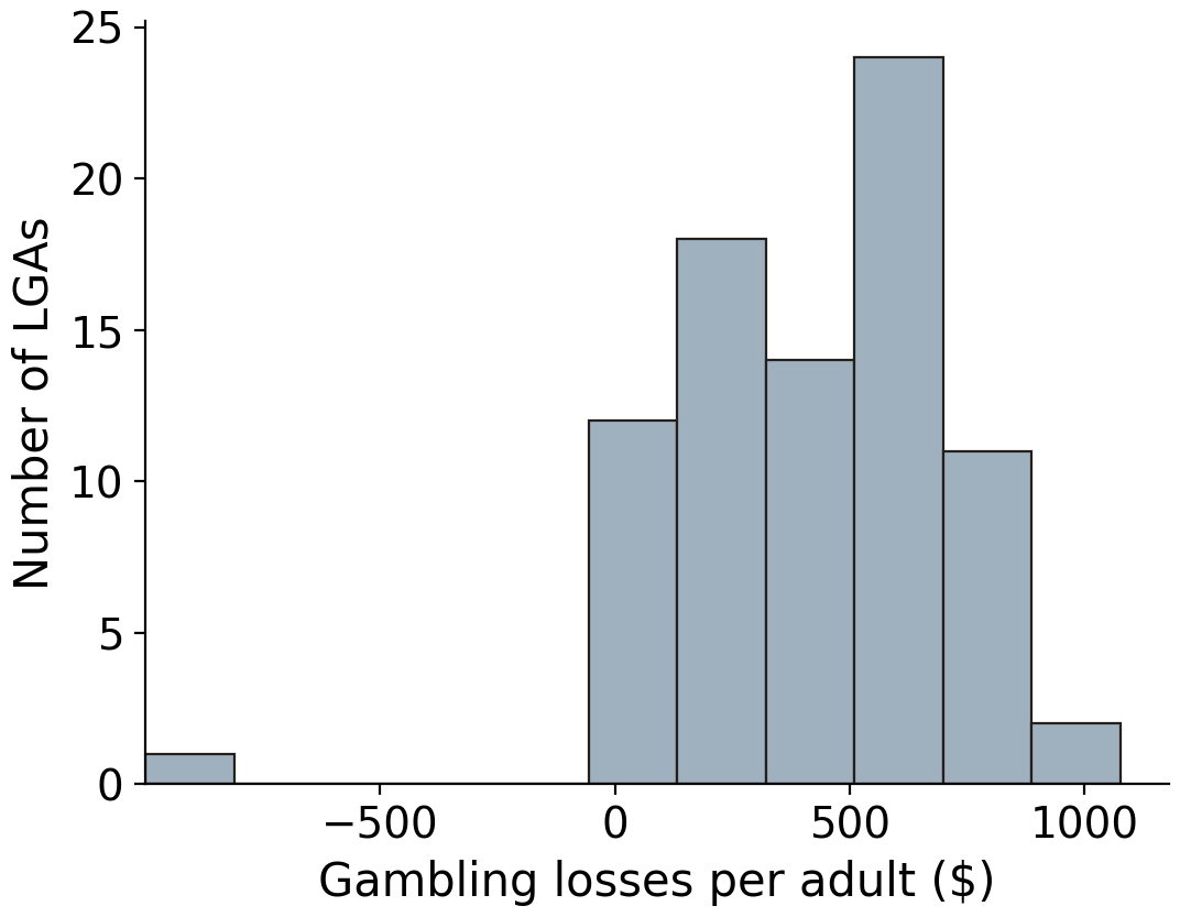
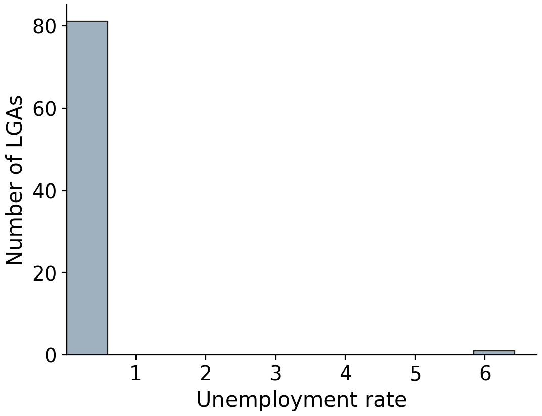
Data: VGCCC 2024, 79 Victorian LGAs, with problems that we planted
One line of Python finds each planted problem
Do messy data change results?
Do the extra variables improve the fit?
Unrestricted: exp_per_adult ~ egm_per_1000 + high_ue + SEIFA_dis_score
Restricted: exp_per_adult ~ egm_per_1000
H_0: \beta_2 = \beta_3 = 0
If the null is true, dropping them should barely hurt the fit
Dropping variables leaves more unexplained
Sum of squared residuals (SSR): what each model leaves unexplained
Restricted SSR: 2,208,120
Unrestricted SSR: 1,848,963
Difference: 359,157
Is 359,157 a lot?
F compares the loss of fit with the noise
Loss of fit per restriction: 359,157 / 2 = 179,579
Noise per degree of freedom: 1,848,963 / 75 = 24,653
F = 179,579 / 24,653 = 7.28
F = \frac{(SSR_r - SSR_{ur})/Q}{SSR_{ur}/(n-k-1)}
We reject the null that both coefficients are 0
median_val = pokies["ue_rate"].median()
pokies["high_ue"] = (pokies["ue_rate"] > median_val).astype(int)
model = ols("exp_per_adult ~ egm_per_1000 + high_ue + SEIFA_dis_score",
            data=pokies).fit()
model.f_test("high_ue = 0, SEIFA_dis_score = 0")
<F test: F=7.284290812093372, p=0.0012851645634963454, df_denom=75, df_num=2>Data: VGCCC 2024, 79 Victorian LGAs
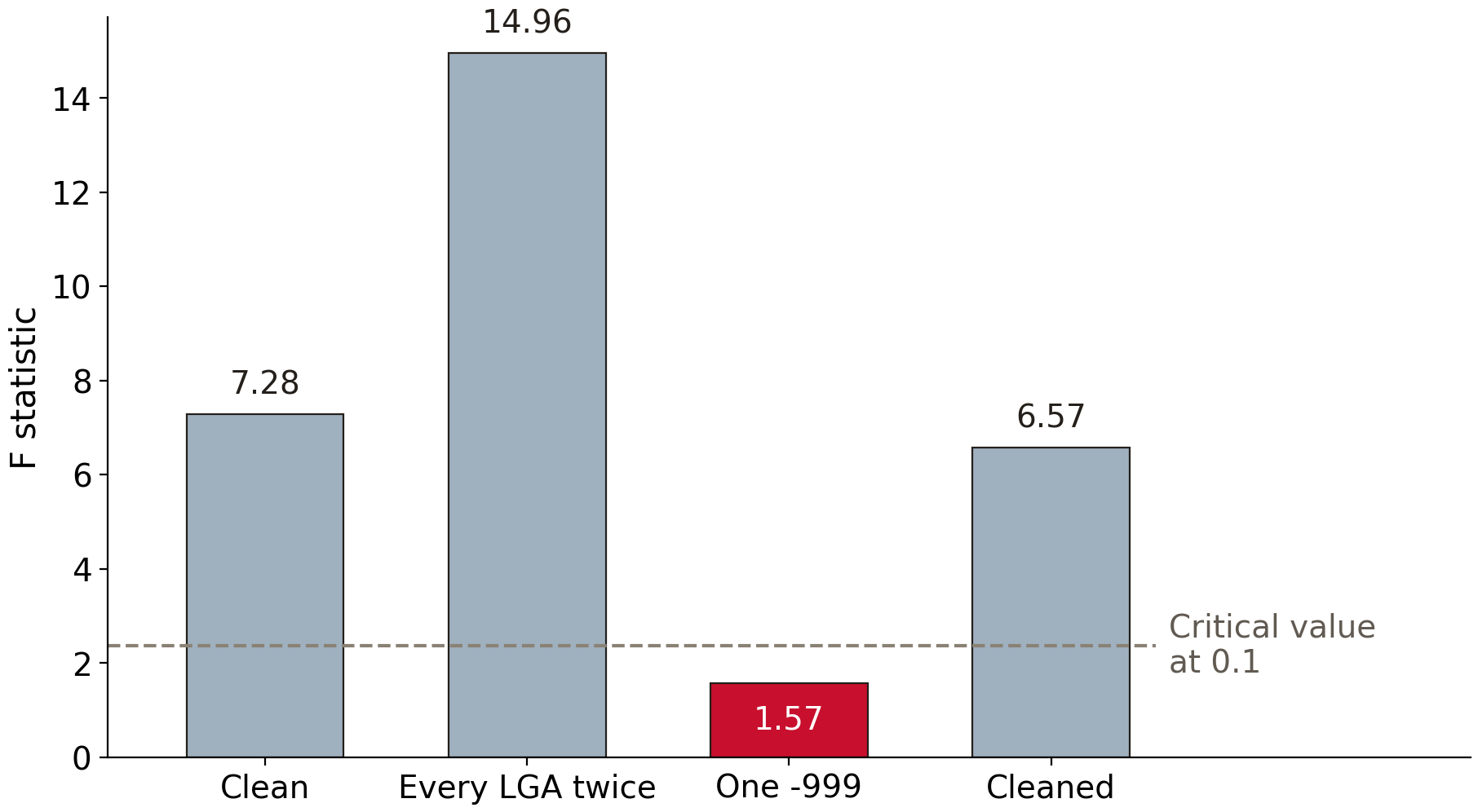
Duplicates make us look more sure than we are
<F test: F=14.95707713416505, p=1.1580534825703107e-06, df_denom=154, df_num=2>Same coefficients, smaller standard errors
high_ue standard error: 25.91, against 37.12
With the -999 left in, we can't reject the null
messy = messy.drop_duplicates()
messy.loc[messy["ue_rate"] > 1, "ue_rate"] = messy["ue_rate"] / 100
# then high_ue, the same model, and f_test
<F test: F=1.5654350799342398, p=0.21574839992285985, df_denom=75, df_num=2>high_ue coefficient: 84.77, against 130.29
With -999 as missing, we reject the null again
<F test: F=6.566531396601032, p=0.002370300275475509, df_denom=74, df_num=2>ols drops Whittlesea, so n = 78
F is larger with duplicates, smaller with -999
Data: VGCCC 2024, 79 Victorian LGAs, with problems that we planted
Before you test, look at your data
describe(): impossible mins and maxes, and the count
histplot(): values far from the rest
duplicated(): rows that appear twice
Next week: diagnostics
Essential Concepts: robust standard errors
Problem set due Friday 16 October
Optional: DIME Analytics Data Handbook, chapter 5