ECON 2041
Introductory Econometrics
How sure are we?
Plan for the semester
1 What is econometrics?
2 Basic mathematical tools
3 Stats fundamentals
4 Stats fundamentals II
5 Simple regression
6 OLS properties & fit
7 Flavors of OLS & OVB Quiz
8 Causality
9 Regression inference
10 Inference, continued PS due 16 Oct
11 Diagnostics
12 Measurement error & IRL
13 Revision
Plan for today
- The rest of the regression table
- Slope sampling distribution
- Testing null hypotheses
- Do the slopes differ?
LET & LEU
- LET (my teaching): closes Friday 9 October, 11 p.m.
- LEU (the unit): Monday 12 October to Sunday 1 November
Fewer datasets, used more times
Personalized feedback on the quiz
Practice questions like the quiz and the final exam
Related topics taught more closely together
The rest of the regression table
We judge how sure we are of the slope
                   coef    std err          t      P>|t|      [0.025      0.975]
--------------------------------------------------------------------------------
Intercept       71.1722     38.992      1.825      0.072      -6.471     148.816
egm_per_1000    78.2968      7.205     10.866      0.000      63.949      92.645
Data: VGCCC 2024, 79 Victorian LGAs
You can follow along in a notebook
https://emiliatjernstrom.com/econ2041/lectures/w09
As usual, it will open directly in Colab
Click Copy to Drive first, so you can save your edits
Slope sampling distribution
In the population, we know the true slope
                 coef    std err          t      P>|t|      [0.025      0.975]
------------------------------------------------------------------------------
escs          43.8472      0.971     45.138      0.000      41.943      45.751
Data: PISA 2022, Australia (OECD), all 12,136 students
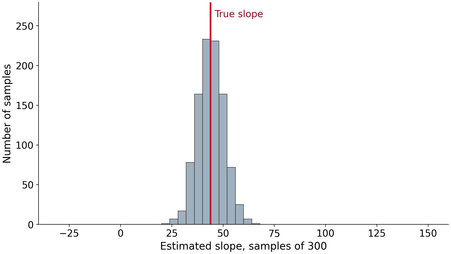
Slope estimate across samples
                 coef    std err          t      P>|t|      [0.025      0.975]
------------------------------------------------------------------------------
escs 42.0037 5.944 7.067 0.000 30.307 53.701Data: PISA 2022, Australia (OECD), samples of 300 students
Sample slopes are centered on the true slope
Data: PISA 2022, Australia (OECD)
The standard error estimates coeff variability
Standard deviation (across 1,000 slopes): 6.4
Standard error (average, across samples): 6.2
In real work, we have one sample and its standard error
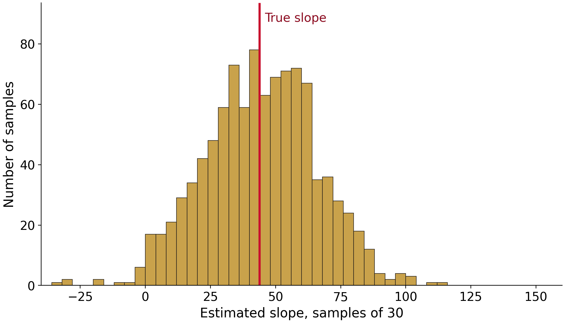
Small samples have more spread-out slopes
Data: PISA 2022, Australia (OECD)
Testing null hypotheses
t is the estimate divided by its standard error
H_0: \beta_1 = 0
t = \frac{\hat{\beta}_1 - 0}{SE(\hat{\beta}_1)} = \frac{78.30}{7.205} = 10.87
We can reject the null of a zero pokie slope
If \beta_1 = 0, how likely is a t at least this far from 0?
Not the probability that \beta_1 = 0
The 95% confidence interval for the slope
\hat{\beta}_1 \pm t^* \times SE(\hat{\beta}_1) = 78.30 \pm 1.99 \times 7.205
Across repeated samples, 95% of confidence intervals contain the true slope
Most confidence intervals contain the slope
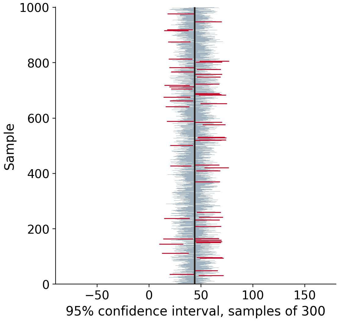
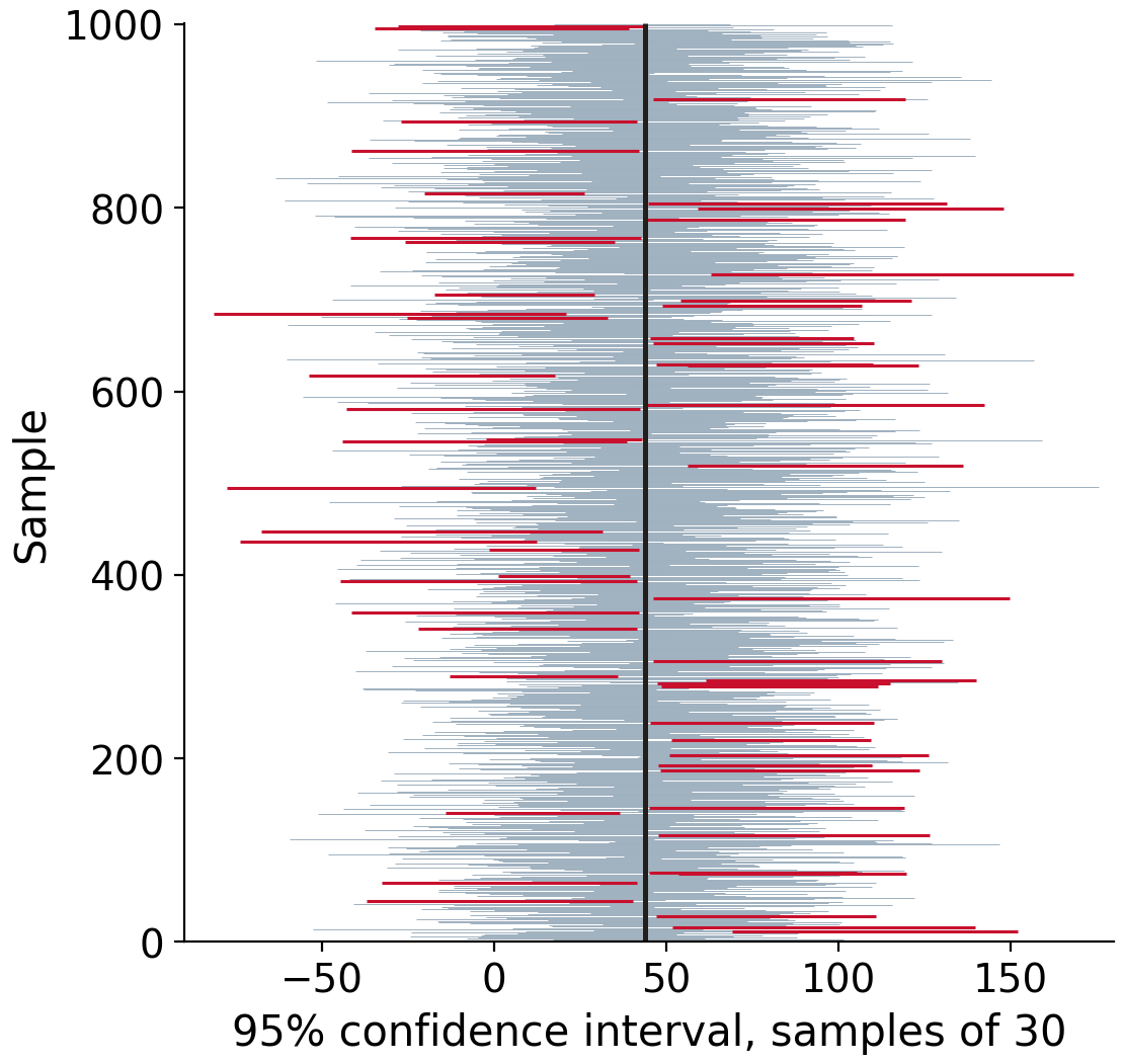
Data: PISA 2022, Australia (OECD); 1,000 samples of 300 (left) and of 30 (right)
Stars in the table mark p-value thresholds
summary_col([model, multi, multi_ue, levels, inter], stars=True, float_format="%.2f",
            model_names=["Simple", "Dummy", "Percent", "3 levels", "Interaction"])
Simple Dummy Percent 3 levels Interaction
----------------------------------------------------------------------------
Intercept 71.17* 16.14 -115.93** 13.27 31.94
(38.99) (38.74) (49.52) (41.58) (47.19)
egm_per_1000 78.30*** 75.87*** 72.83*** 76.93*** 72.33***
(7.21) (6.67) (6.33) (6.60) (8.98)
high_ue 134.71*** 96.73
(35.30) (73.30)
ue_pct 61.18***
(11.85)
C(ue_cat)[T.medium] 28.53
(42.57)
C(ue_cat)[T.high] 167.05***
(42.55)
egm_per_1000:high_ue 7.99
(13.50)
R-squared 0.61 0.67 0.71 0.68 0.67
R-squared Adj. 0.60 0.66 0.70 0.67 0.66* p < 0.1 ** p < 0.05 *** p < 0.01 (standard errors)
Do the slopes differ?
Can't reject equal slopes by unemployment
                           coef    std err          t      P>|t|      [0.025      0.975]
----------------------------------------------------------------------------------------
Intercept               31.9430     47.186      0.677      0.501     -62.056     125.942
egm_per_1000            72.3339      8.976      8.058      0.000      54.453      90.215
high_ue                 96.7287     73.302      1.320      0.191     -49.296     242.753
egm_per_1000:high_ue     7.9900     13.496      0.592      0.556     -18.896      34.876
Data: VGCCC 2024, 79 Victorian LGAs
Not rejecting isn't proof of equal slopes
95% confidence interval for the difference in slopes: −18.9 to 34.9
A difference of 0 is inside it
So is a high-unemployment slope $30 steeper
The ESCS slope is smaller for girls than for boys
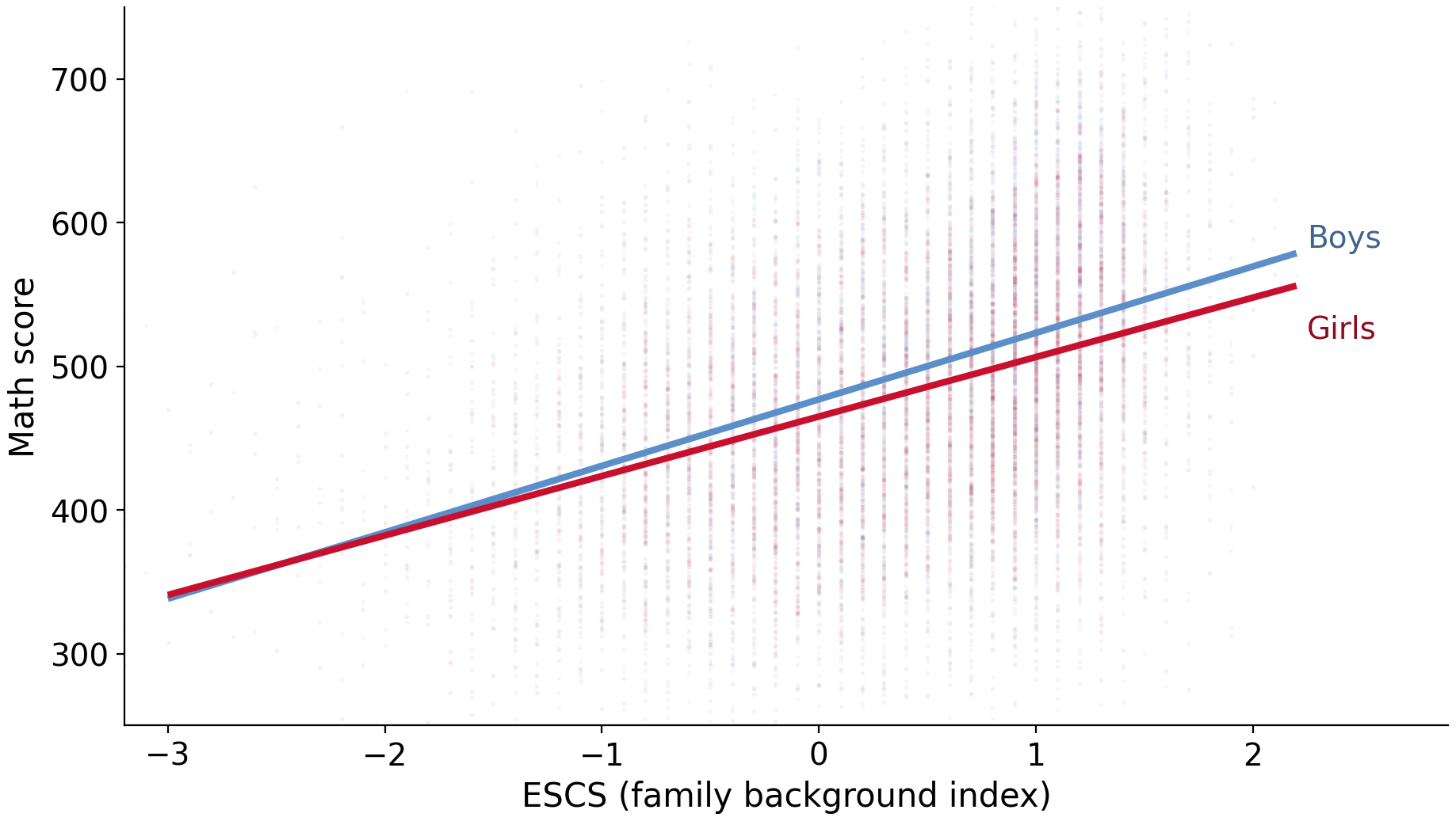
Data: PISA 2022, Australia (OECD)
With all the students, we reject equal slopes
pisa["female"] = (pisa["gender"] == "female").astype(int)
ols("math ~ escs * female", data=pisa).fit()
coef std err t P>|t| [0.025 0.975]
-------------------------------------------------------------------------------
Intercept 477.0806 1.234 386.632 0.000 474.662 479.499
escs 46.2714 1.353 34.209 0.000 43.620 48.923
female -11.9517 1.767 -6.763 0.000 -15.416 -8.488
escs:female -4.8629 1.937 -2.510 0.012 -8.661 -1.065Data: PISA 2022, Australia (OECD), all 12,136 students
At n = 300, we usually can't reject equal slopes
All 12,136 students: p-value 0.012, reject equal slopes
1,000 samples of 300 students: p-value below 0.1 in 12% of them
Data: PISA 2022, Australia (OECD)
Small p-values don't make slopes causal
Pokie slope: p-value 0.000
Pokies aren't randomly assigned to LGAs
Omitted variable bias is a separate problem from sampling variation
Next week: joint tests
Essential Concepts: joint tests and the F test
Problem set due Friday 16 October