Gallery 1: math & reading
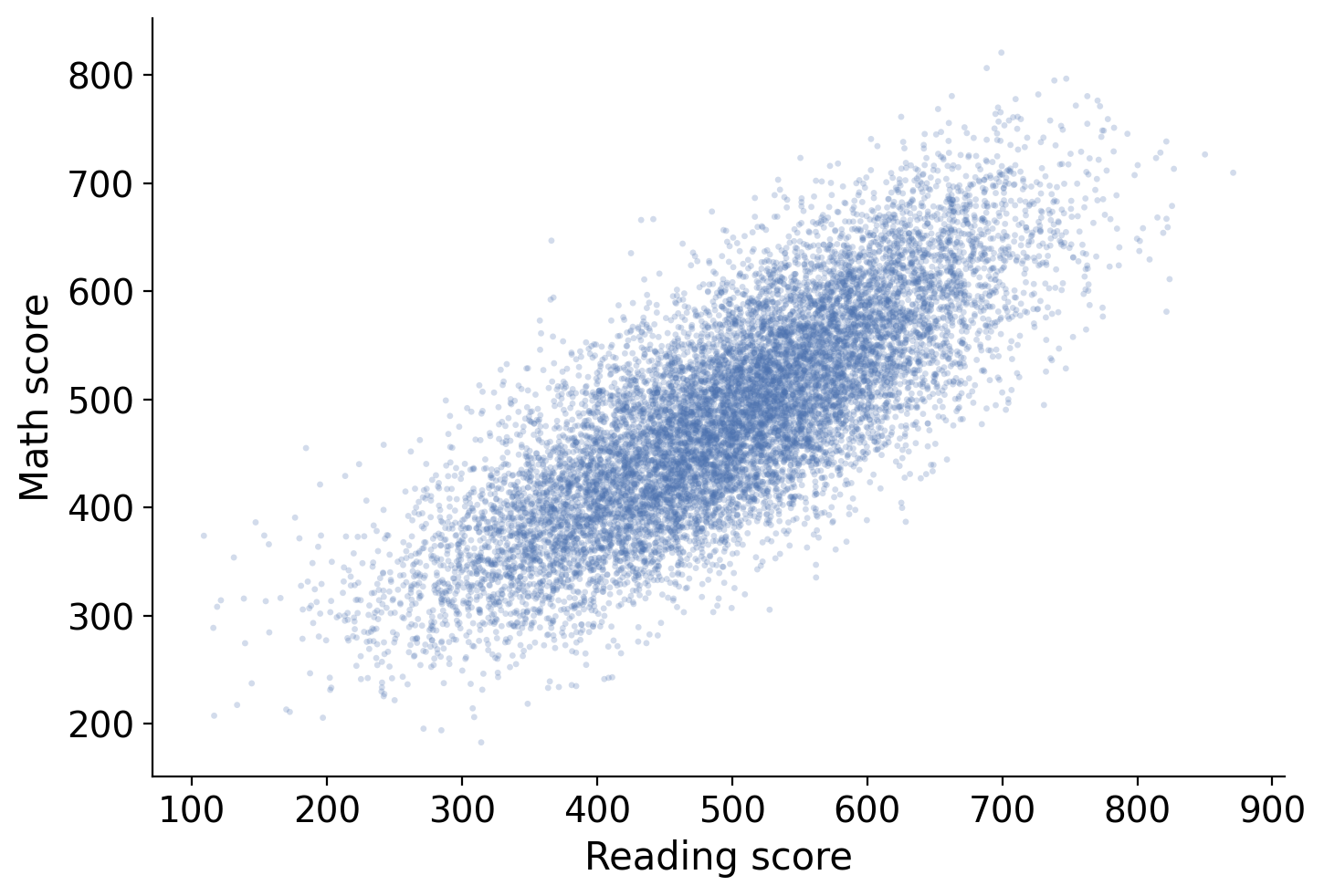
Data: PISA 2022, Australia (OECD)
Gallery 1: math & reading
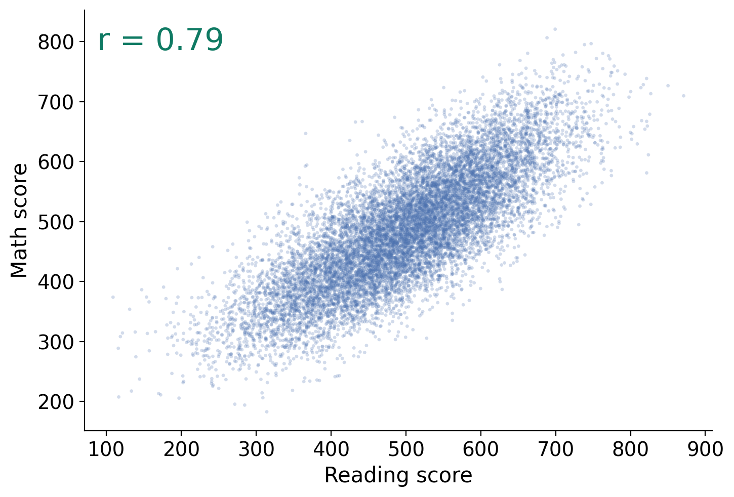
Data: PISA 2022, Australia (OECD)
Gallery 2: math & socio-economic status
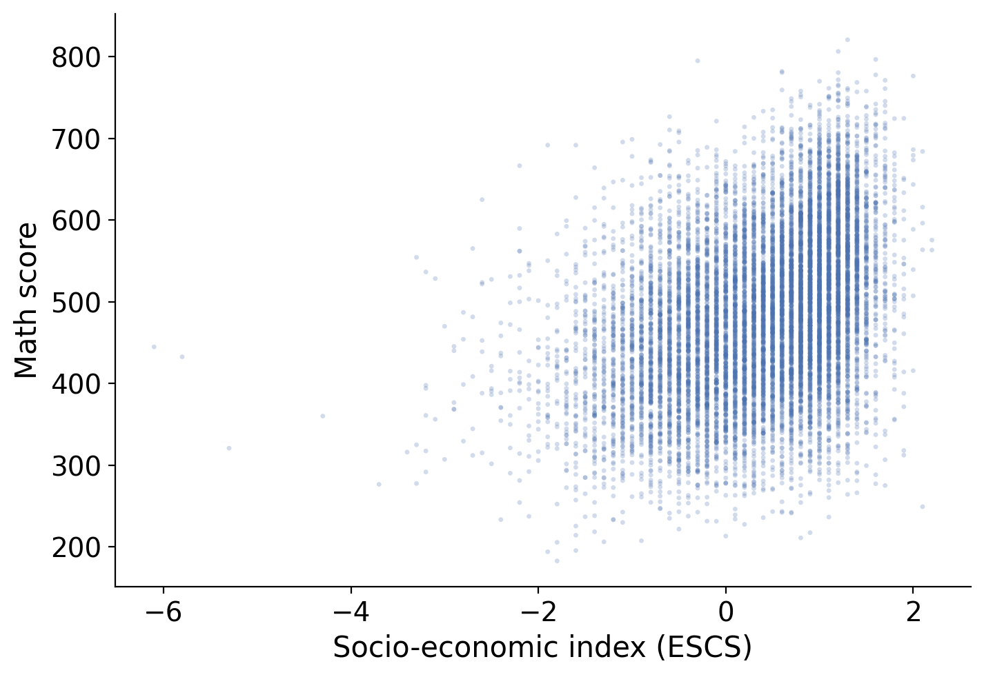
Data: PISA 2022, Australia (OECD)
Gallery 2: math & socio-economic status
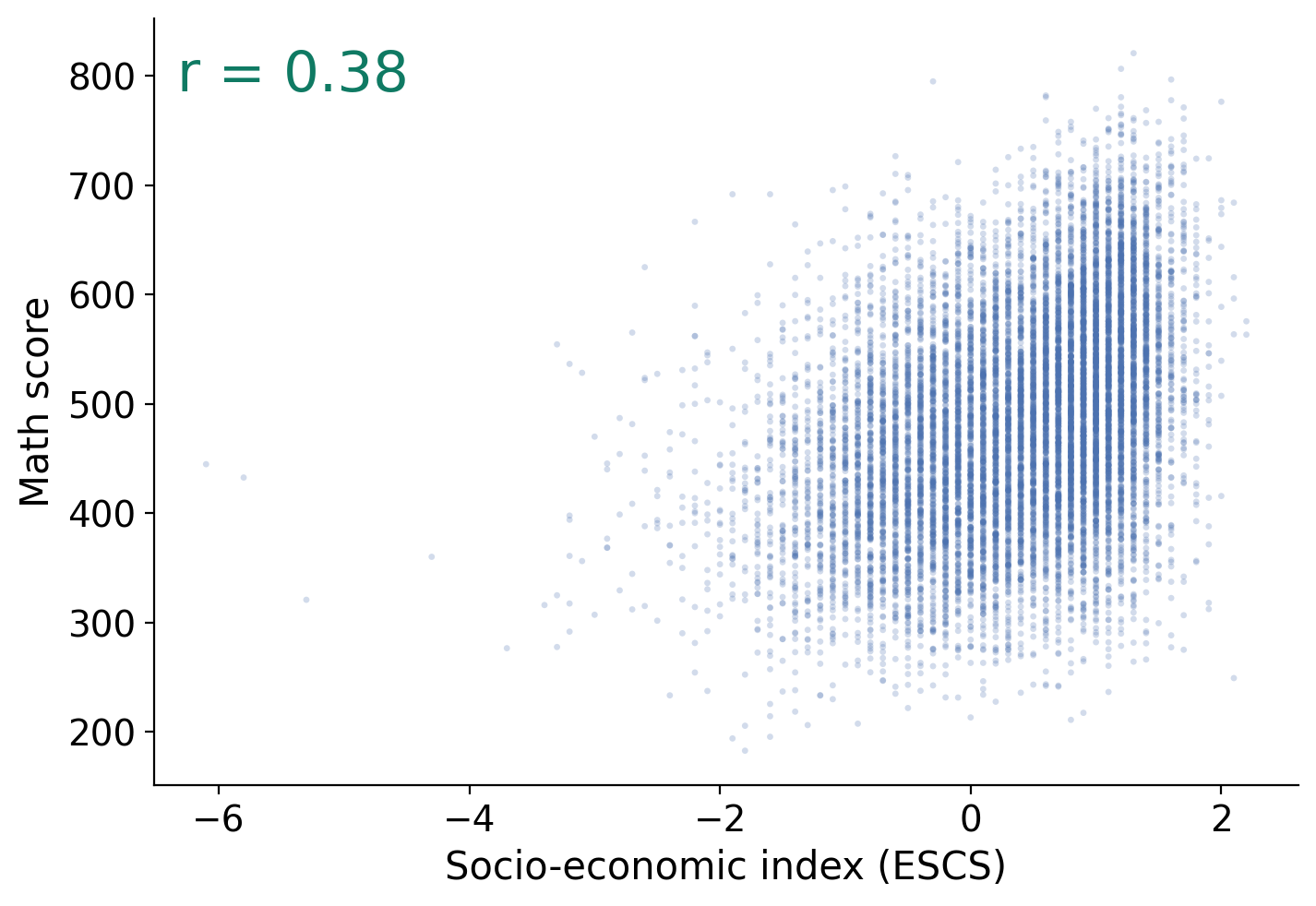
Data: PISA 2022, Australia (OECD)
Gallery 3: simulated data
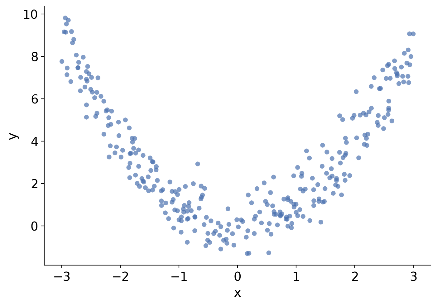
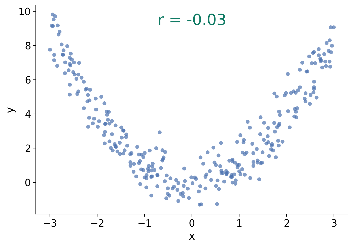
Gallery 3: simulated data
Math vs. socio-economic status (N=300)
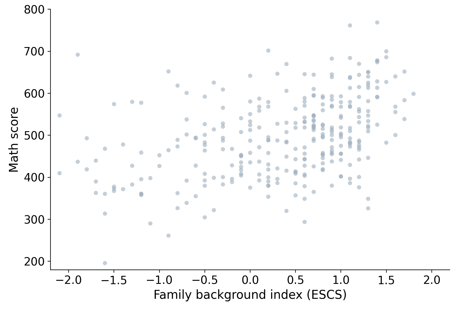
Data: PISA 2022, Australia (OECD), 300 students drawn at random
Step 1: find the two means
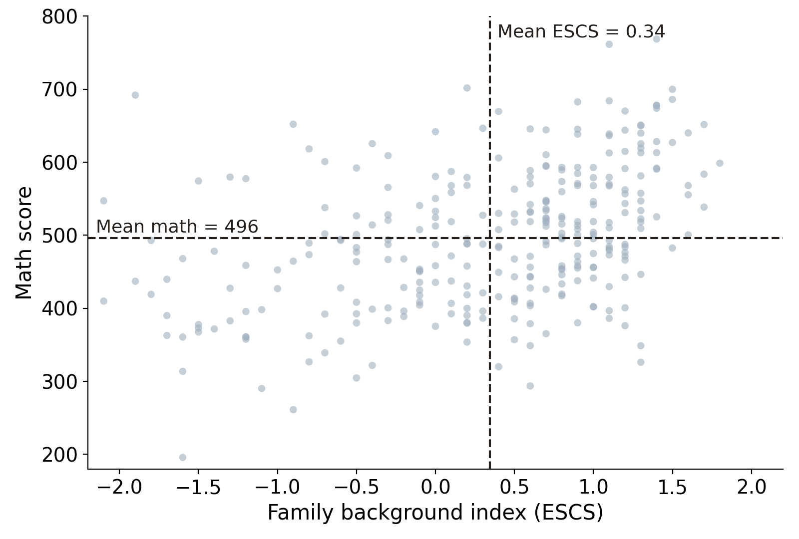
Data: PISA 2022, Australia (OECD), 300 students drawn at random
Step 2: measure deviations for each student
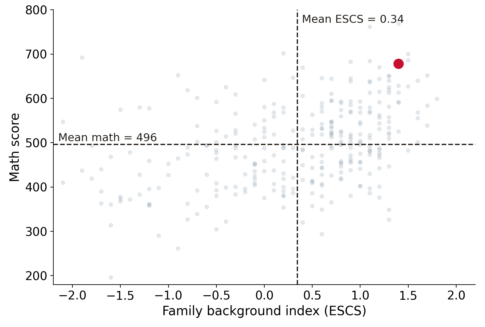
Data: PISA 2022, Australia (OECD), 300 students drawn at random
Step 2: find the X-deviation
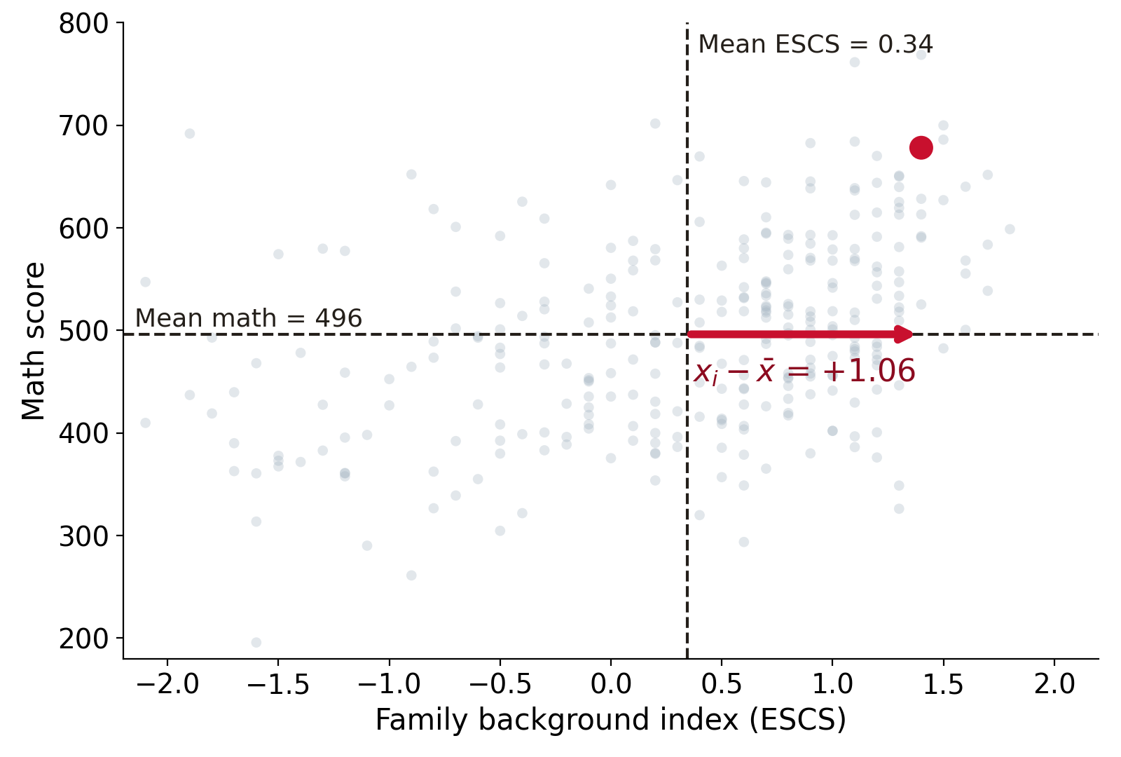
Data: PISA 2022, Australia (OECD), 300 students drawn at random
Step 2: find the Y-deviation
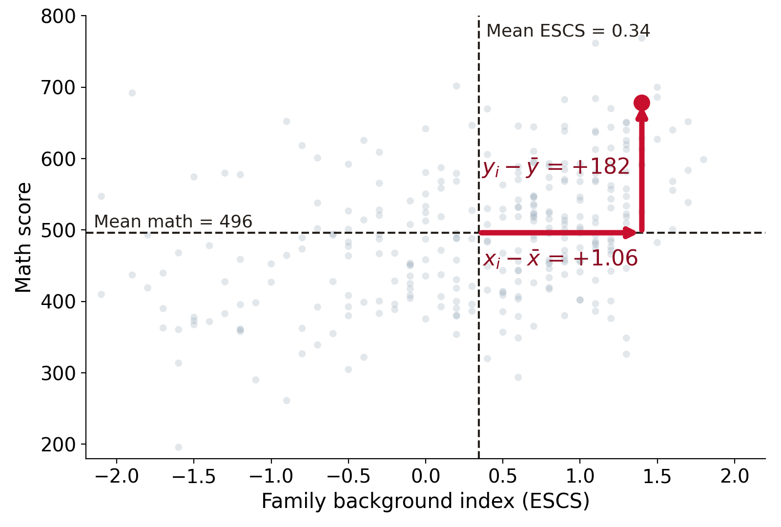
Data: PISA 2022, Australia (OECD), 300 students drawn at random
Step 3: multiply & sum
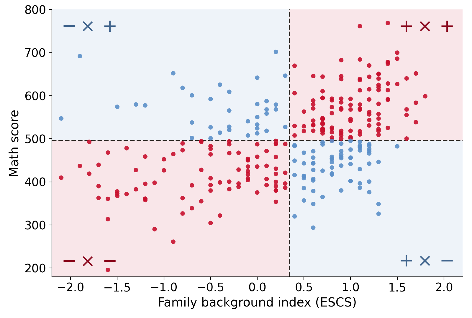
Data: PISA 2022, Australia (OECD), 300 students drawn at random
Step 3: multiply & sum
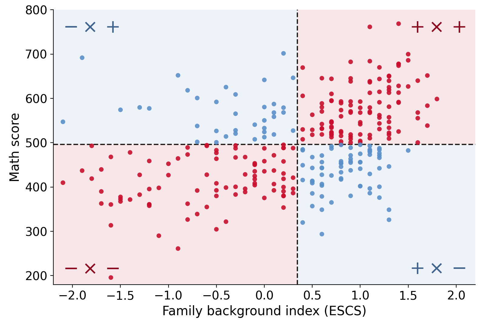
+14,520
positive products
-4,046
negative products
Data: PISA 2022, Australia (OECD), 300 students drawn at random
Fit the line
https://emiliatjernstrom.com/econ2041/portal.html

Average math score for each level of ESCS
Data: PISA 2022, Australia (OECD), 300 students drawn at random
Average math score for each level of ESCS
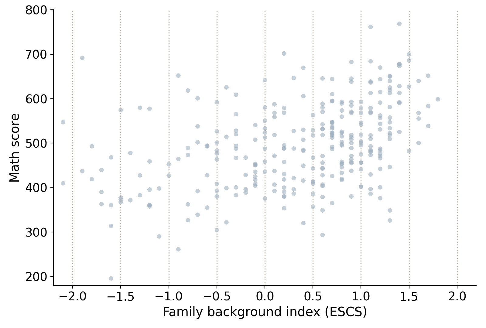
Data: PISA 2022, Australia (OECD), 300 students drawn at random
One slice, one estimated conditional mean
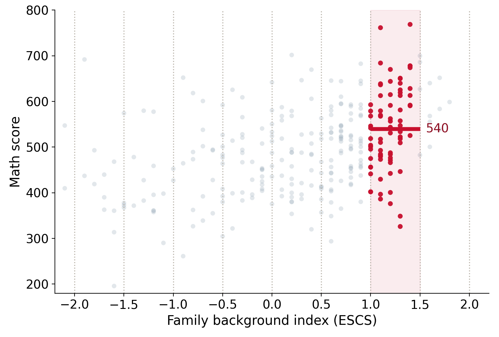
Data: PISA 2022, Australia (OECD), 300 students drawn at random
One slice, one estimated conditional mean
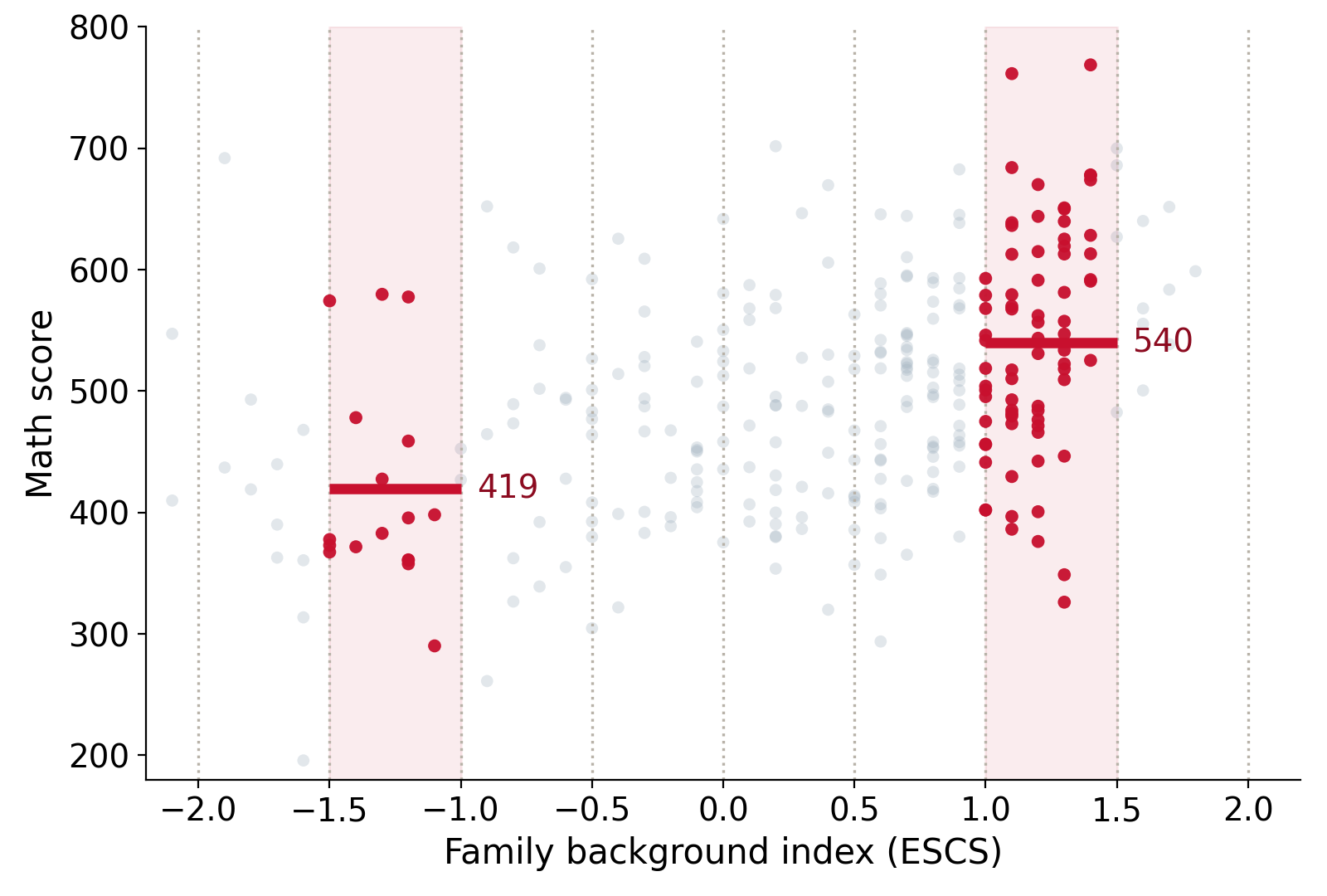
Data: PISA 2022, Australia (OECD), 300 students drawn at random
Slice means estimate the conditional mean
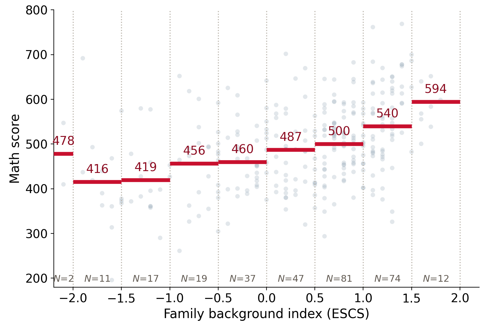
Data: PISA 2022, Australia (OECD), 300 students drawn at random
Summarize conditional means with a line
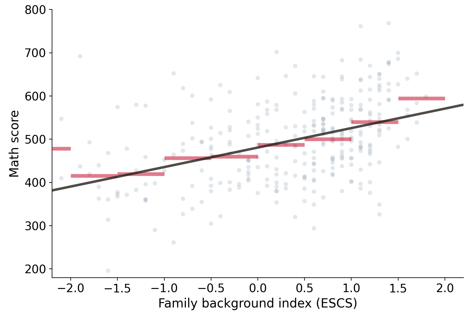
Data: PISA 2022, Australia (OECD), 300 students drawn at random
The population line is the conditional mean
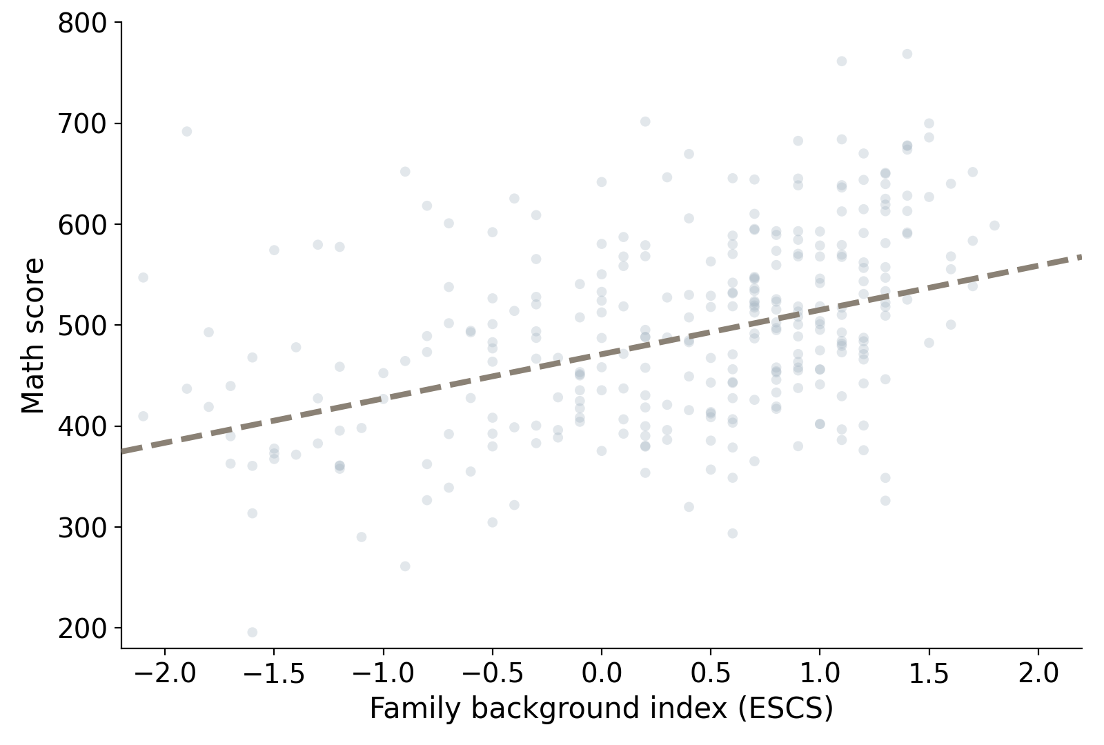
E[Y \mid X] = \beta_0 + \beta_1 X
Data: PISA 2022, Australia (OECD); dashed line fitted on all 12,136 students
An error is the gap from the population line
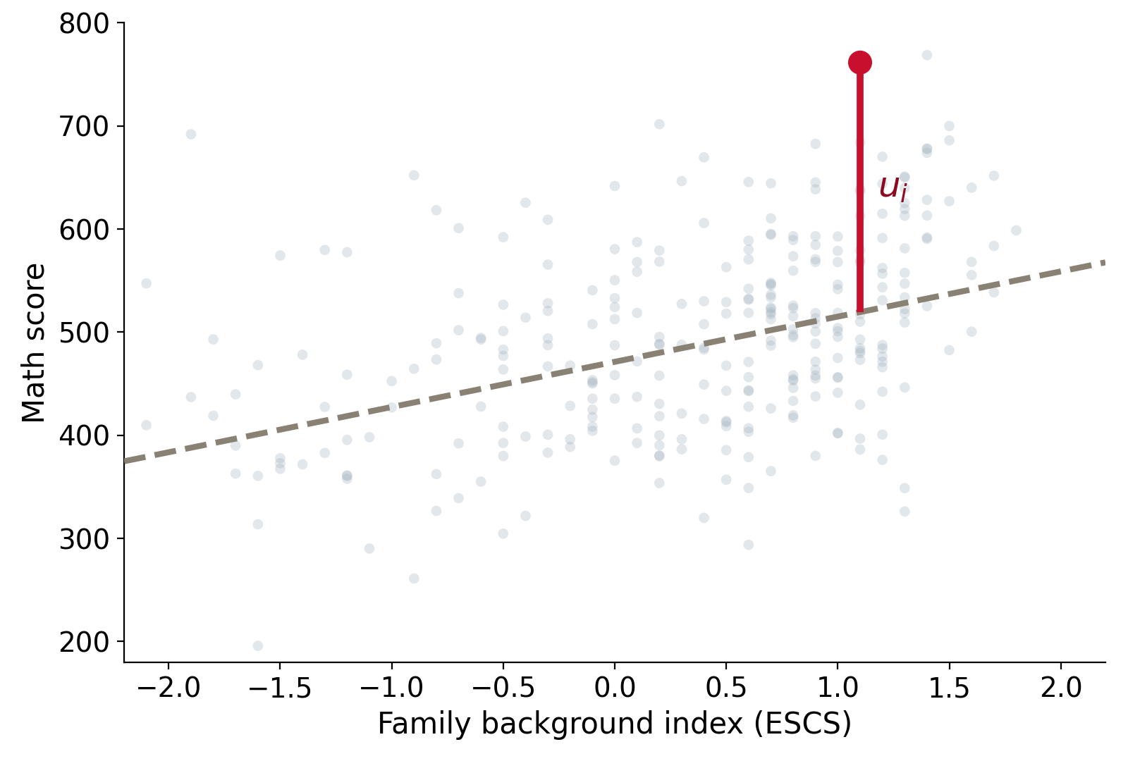
y_i = \beta_0 + \beta_1 x_i + u_i
Data: PISA 2022, Australia (OECD); dashed line fitted on all 12,136 students
The sample gives us a fitted line
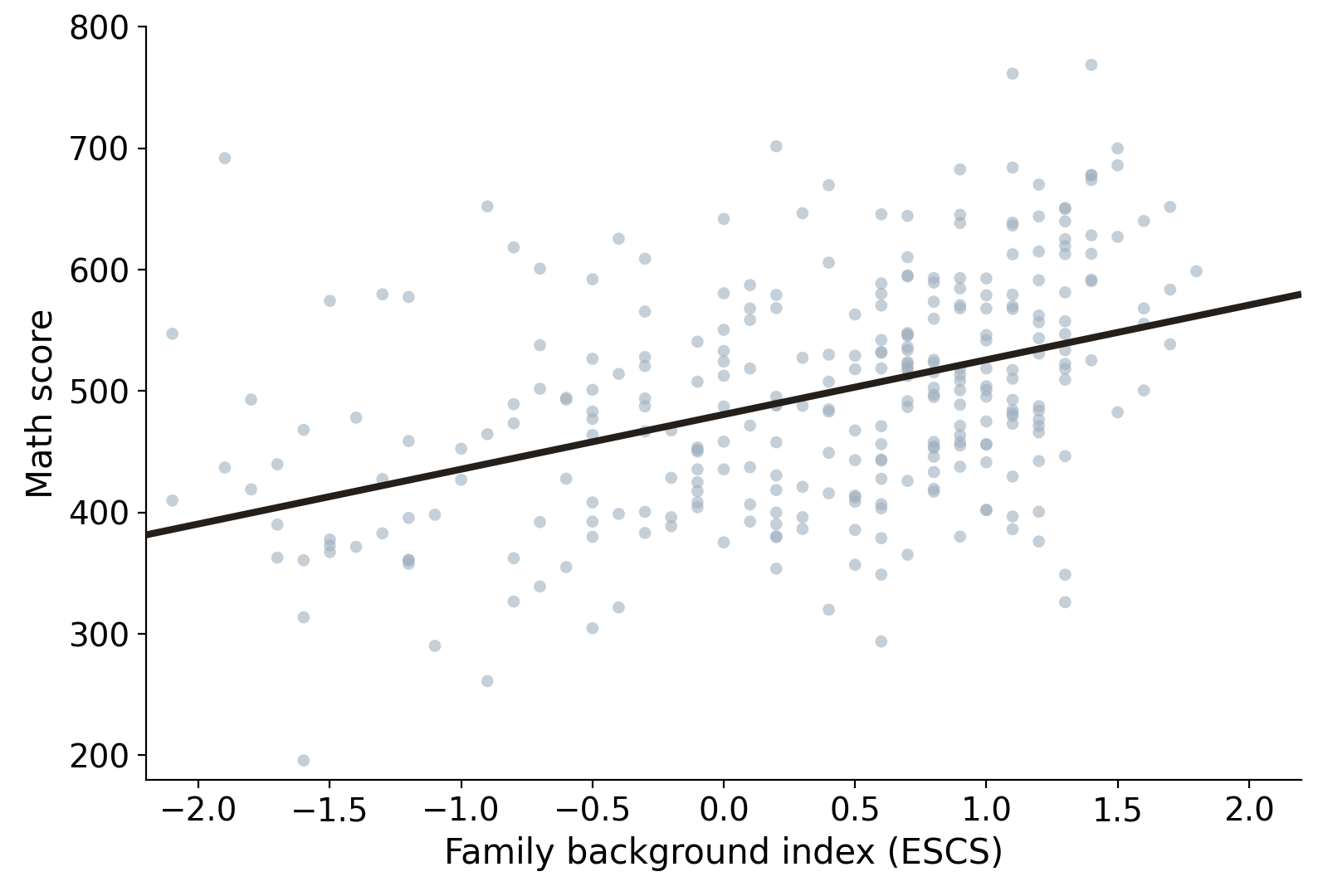
\hat{y} = \hat{\beta}_0 + \hat{\beta}_1 x = 481 + 45x
Data: PISA 2022, Australia (OECD), 300 students drawn at random
The sample gives us a fitted line
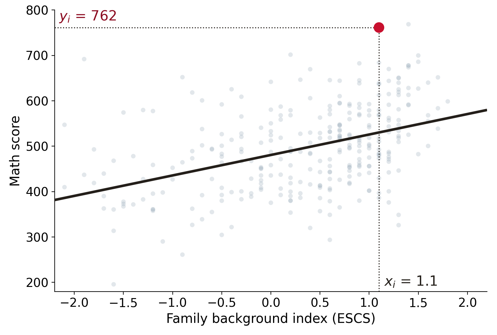
Data: PISA 2022, Australia (OECD), 300 students drawn at random
The line's prediction for student i
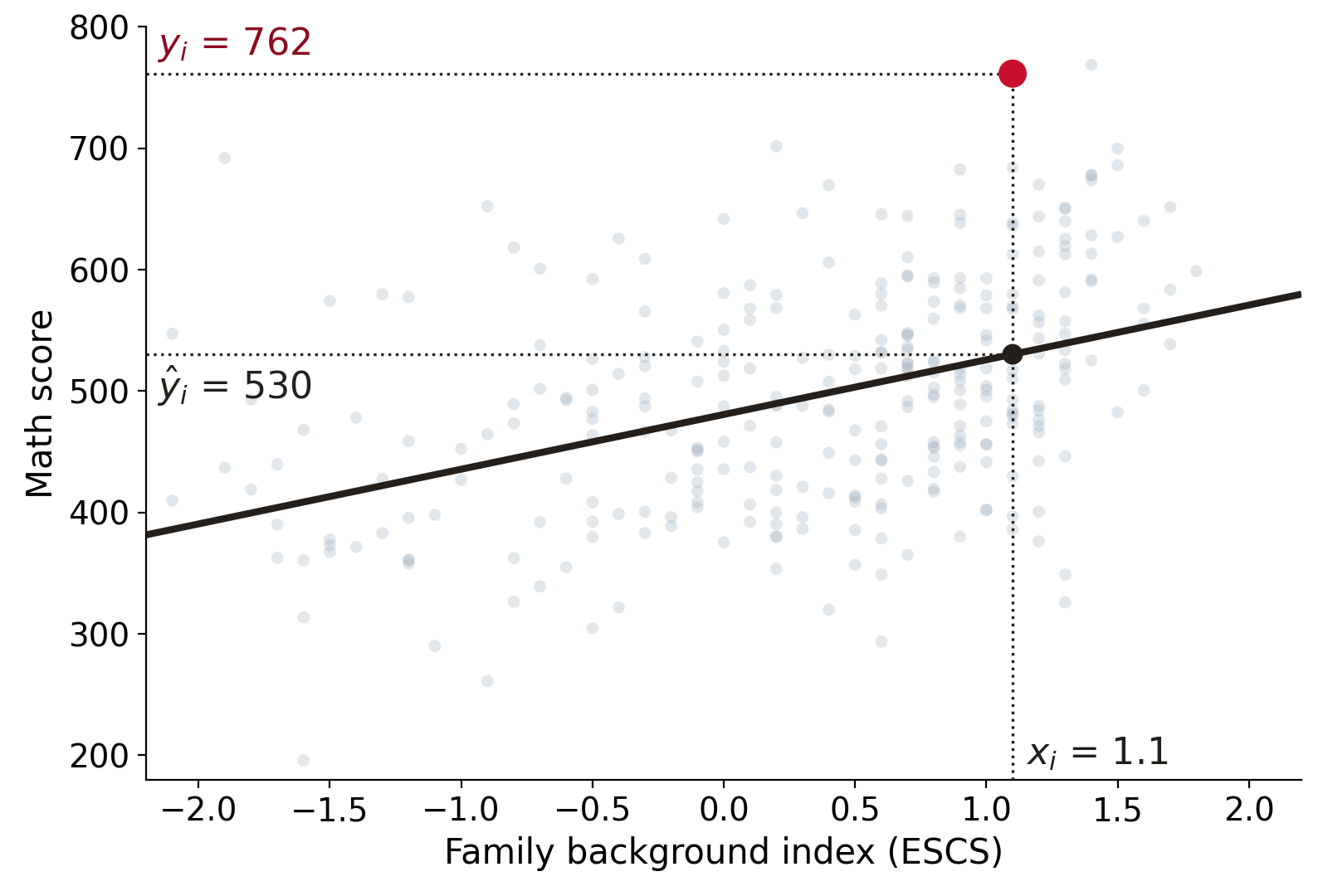
Data: PISA 2022, Australia (OECD), 300 students drawn at random
This gap is called the residual
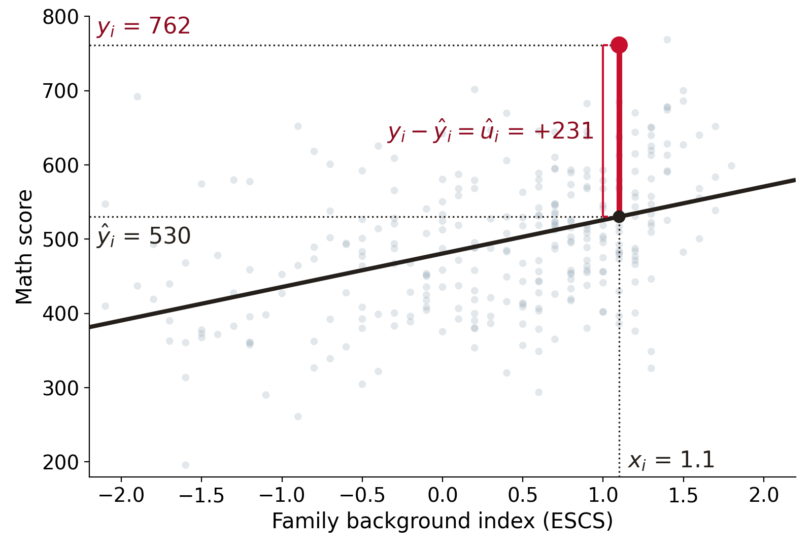
Data: PISA 2022, Australia (OECD), 300 students drawn at random
This gap is called the residual
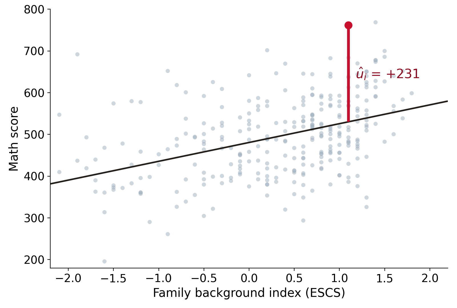
Data: PISA 2022, Australia (OECD), 300 students drawn at random
This gap is called the residual
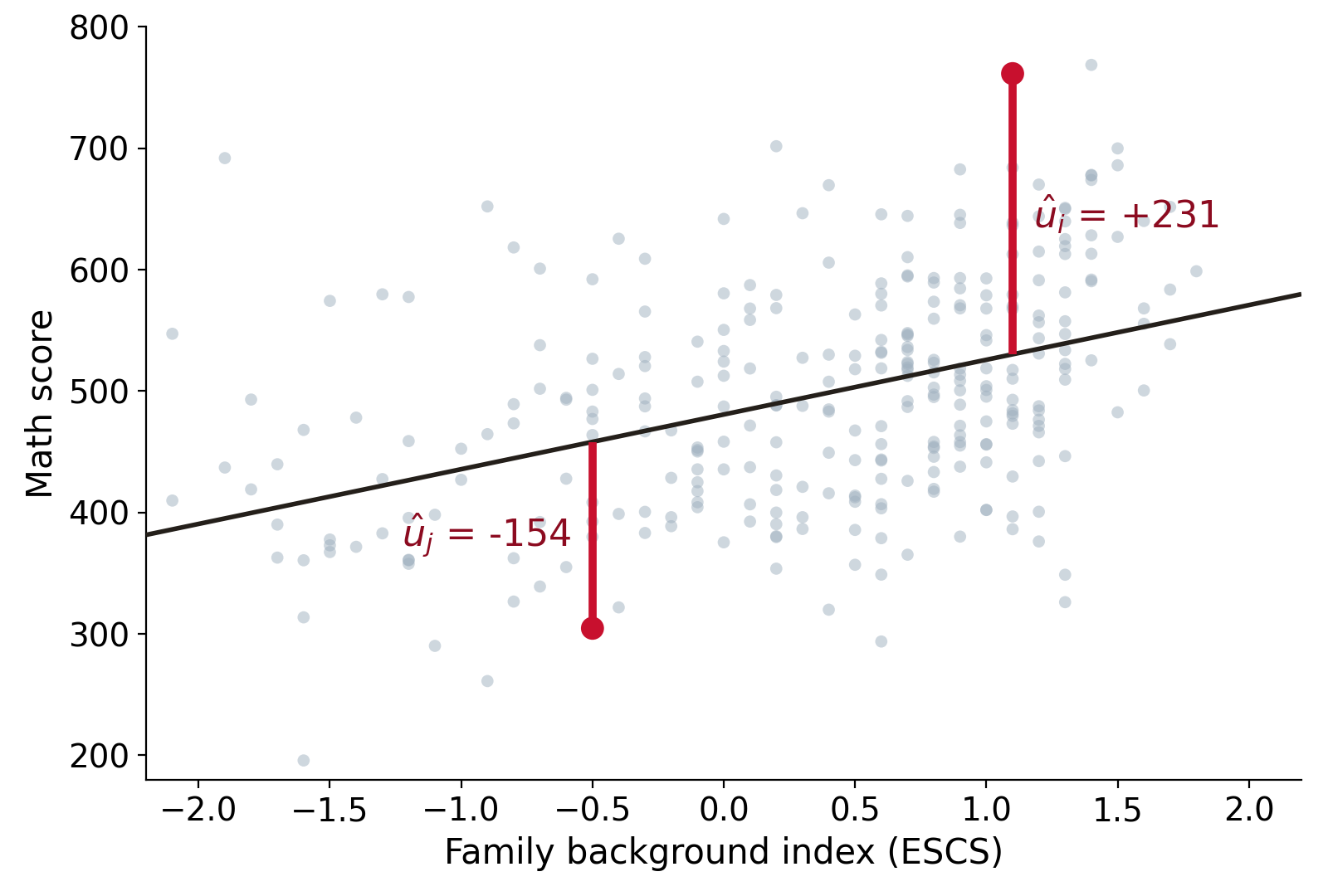
Data: PISA 2022, Australia (OECD), 300 students drawn at random
The residuals: what our summary leaves out
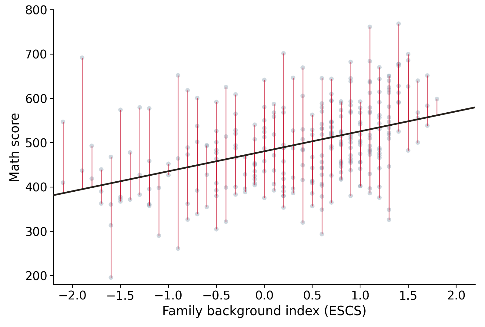
Data: PISA 2022, Australia (OECD), 300 students drawn at random
Minimize the sum of squared residuals
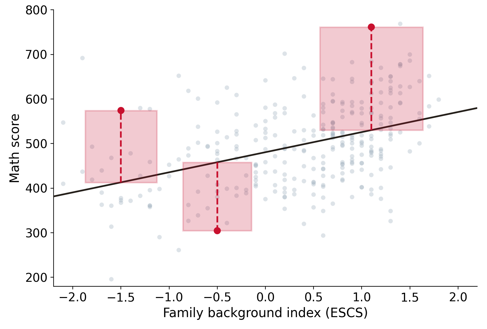
Data: PISA 2022, Australia (OECD), 300 students drawn at random
Squared residuals, flat line
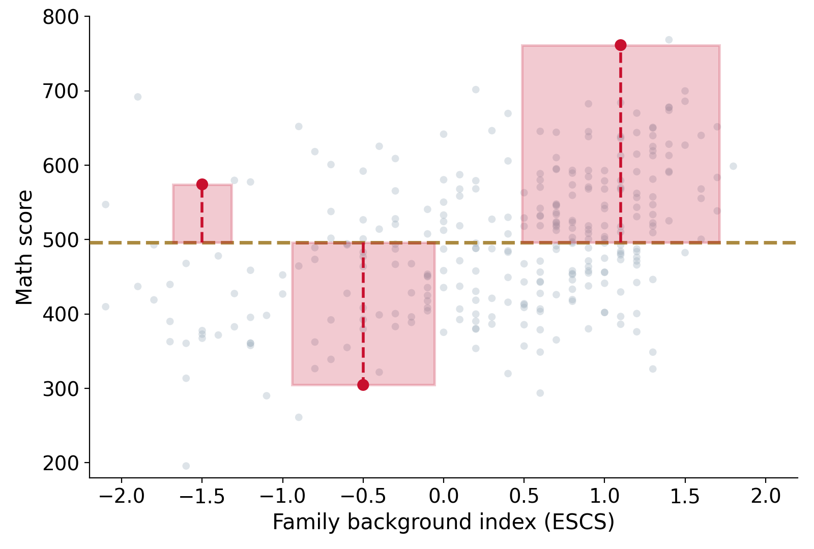
Data: PISA 2022, Australia (OECD), 300 students drawn at random
Squared residuals, steep line
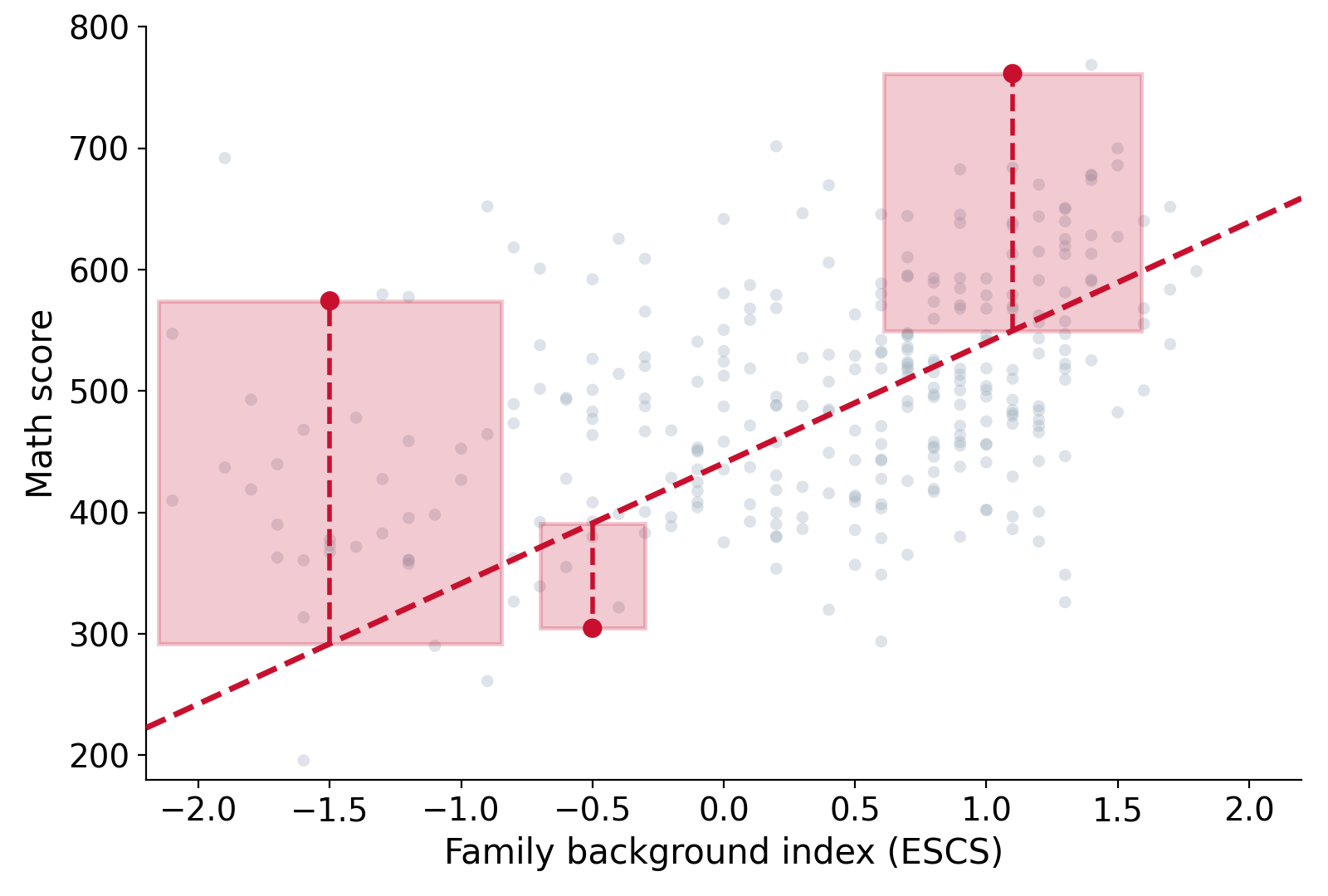
Data: PISA 2022, Australia (OECD), 300 students drawn at random
Squared residuals, shallow line
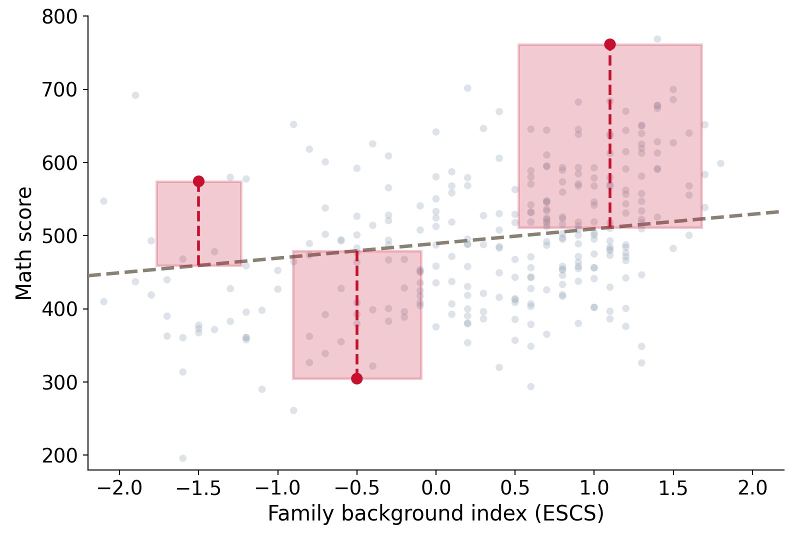
Data: PISA 2022, Australia (OECD), 300 students drawn at random
Least squares: the smallest total area
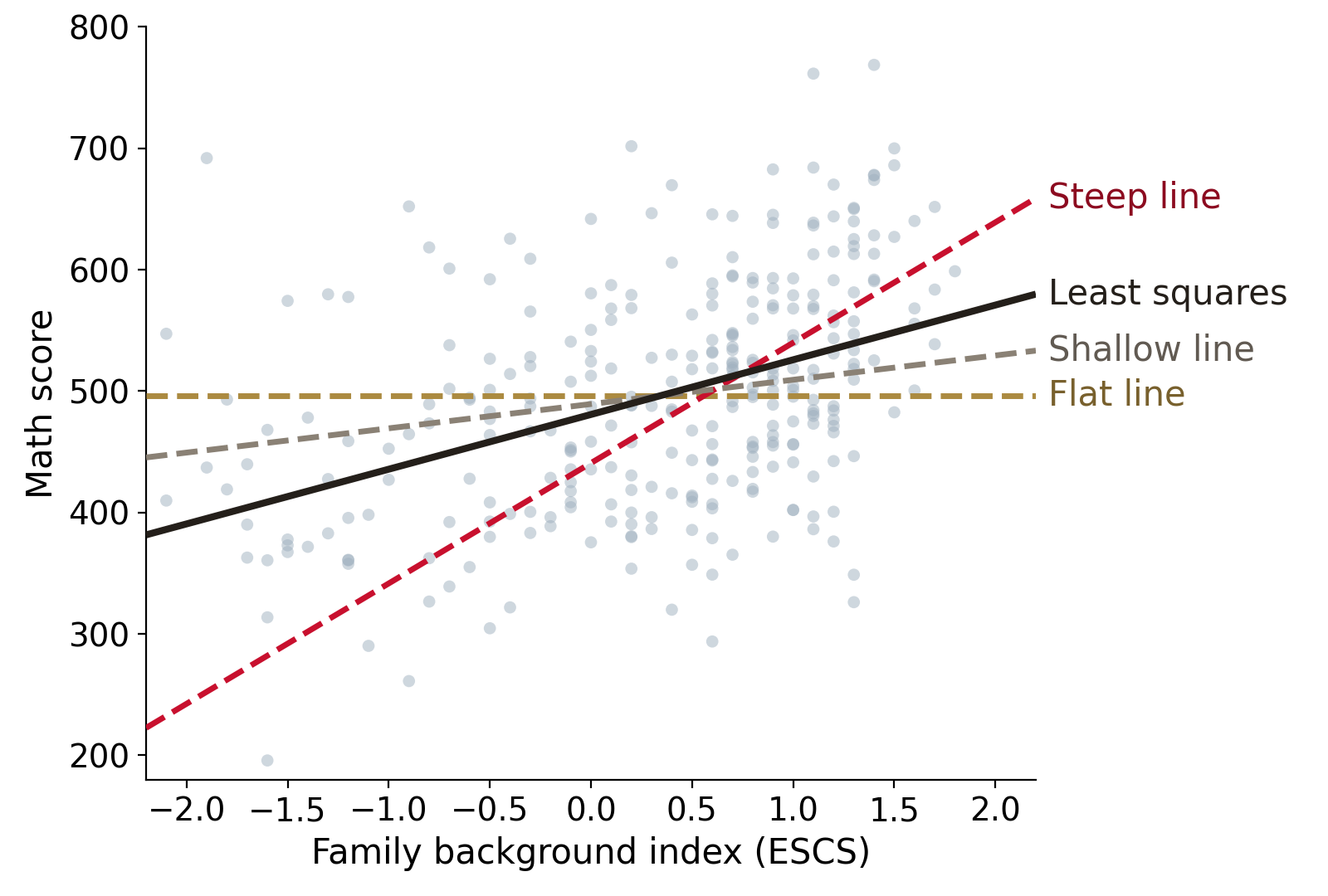
Data: PISA 2022, Australia (OECD), 300 students drawn at random
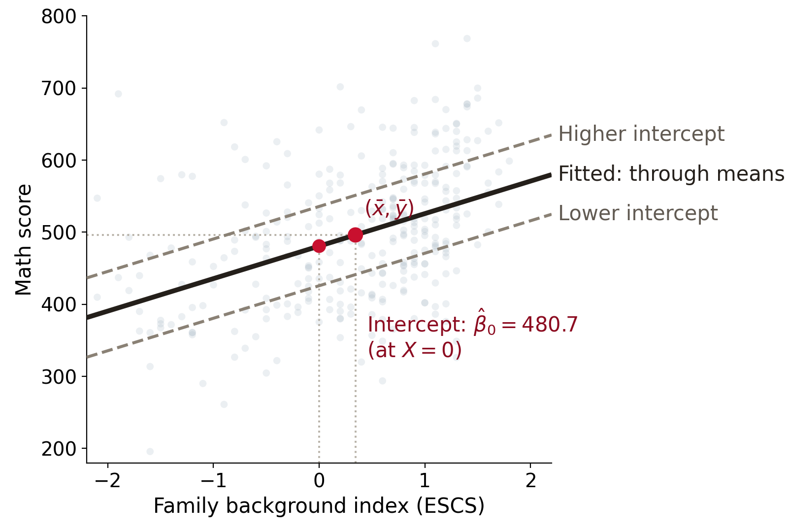
The intercept anchors the line at the means
\bar{y} = \hat{\beta}_0+\hat{\beta}_1\bar{x}
\hat{\beta}_0 = \bar{y}-\hat{\beta}_1\bar{x}
\begin{aligned} &=496.2-45.07(0.343)\\ &=\color{#c8102e}{480.7} \end{aligned}
Small samples can move the fitted line
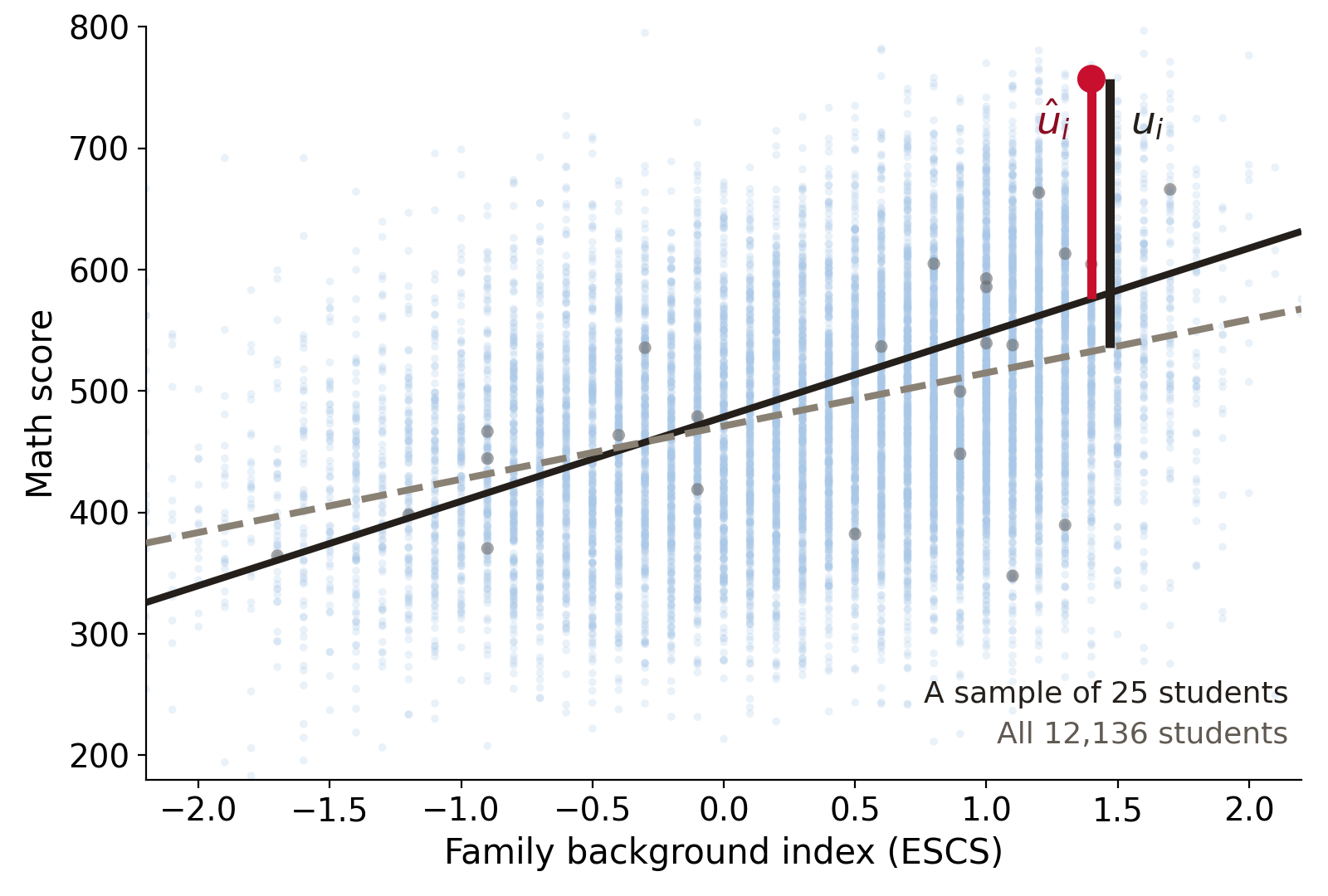
Data: PISA 2022, Australia (OECD); dashed line fitted on all 12,136 students, solid line on a sample of 25